
]>
8
Electromagnetic Modeling of Complex Materials*
The models we used till now assumed that the electromagnetic parameters σ, μ, and ε are scalar constants. In this section, we examine the circumstances under which the electromagnetic parameters are not scalar constants. In particular, we study the frequency dependence of the dielectric constant. In Section 8.1, we first study the interaction of an external electric field with a dielectric material by considering a volume of electric dipoles in free space. In Section 8.2, we study the frequency dependence of a dielectric material by considering a mechanical equivalent of an atom in a dielectric.
8.1Volume of Electric Dipoles
Let us briefly revise the concept of a dipole. An elementary electric dipole is constructed by a negative and a positive charges of equal value separated by a small distance d (Figure 8.1).

FIGURE 8.1
Electric dipole.
The dipole moment p of this system is given by
The potential fields Φp due to such a dipole, when r ≫ d, is given by
and the electric field is given by
For a more general distribution of volume charges in a localized volume, where the total charge is zero, the dipole moment (Figure 8.2) is given by
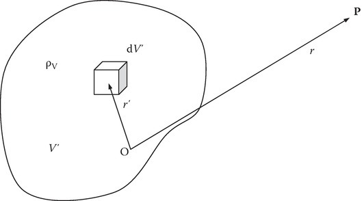
FIGURE 8.2
Dipole moment for a general distribution of volume charges.
The potential due to a volume of dipoles in V′ of dipole moment P per unit volume, also called polarization vector (C/m2) (see Figure 8.3), is given by
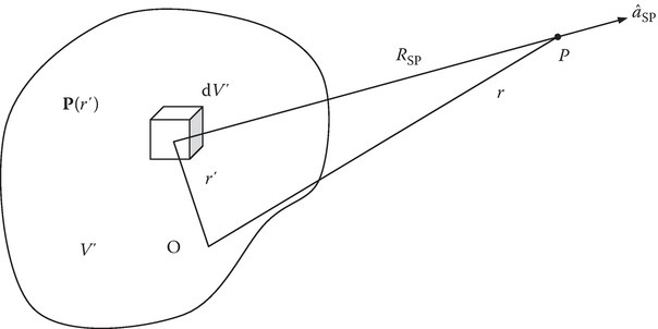
FIGURE 8.3
Volume of dipoles of polarization P.
Equation 8.5 may be transformed into
By comparing Equation 8.6 with similar expressions for potential due to monopole distributions, the following equivalence may be drawn: a volume of dipoles of dipole moment density P is equivalent to a monopole volume charge of density ρVb and a surface charge density ρSb:
(see Figure 8.4).
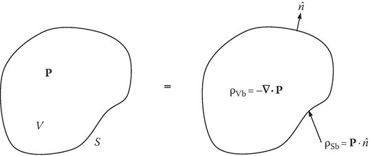
FIGURE 8.4
Equivalence of volume of electric dipoles with monopole distributions.
Gauss’s law in free space with volume of dipoles can be written as
where ρV is the volume charge density due to free charges and ρVb is an equivalent volume charge density due to the volume of dipoles.
By substituting Equation 8.7 into Equation 8.9, we obtain
Let us denote
For linear materials, P is proportional to E and let us write this linear dependence in terms of electric susceptibility χe:
Substituting Equation 8.12 into Equation 8.11, we obtain
where
and is called relative permittivity.
8.2Frequency-Dependent Dielectric Constant
Under the influence of an electric field, the positive and negative charges inside each atom are displaced from their equilibrium position. Since the mass of the nucleus M is much larger than that of an electron m, M ≫ m, the positive charge is assumed to be stationary. The electron moves and exhibits a friction coefficient ν. The mechanical equivalence of the system is shown [1] in Figure 8.5.
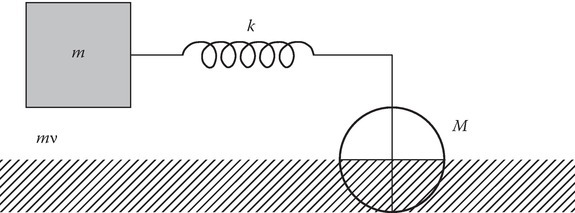
FIGURE 8.5
Mechanical equivalence of an atom in a dielectric.
When a time-harmonic electric field of angular frequency ω, E = E0 ejωt, is applied to the atom, the force equation is given by
where x is the position of the electron relative to the atom. To find the particular solution, let x = x0 ejωt, then
where
and q is the absolute value of the charge and m is the mass of the electron. The displacement of the charge centers gives rise to a dipole moment p = −qx. If there are N dipoles created per unit volume, then the polarization P, which is the dipole moment per unit volume, is given by
The electric susceptibility χe defined by P = ε0χeE can be computed as
The complex dielectric constant εr = εp = 1 + χe = n2. Because of the presence of ν, εr and n are complex. The parameter ν is called the collision frequency and has the unit of radians/second. Denoting the numerator of the right-most part of Equation 8.20 by ω2p, the dielectric (constant) function is
where
In simple metals, there are free electrons that are not bound (k = 0) but are free to move, that is, ω0 = 0, and
On the other hand, for some dielectrics, there are multiple resonances and for such materials, the most general form of the dielectric function is given by
In the above, ε∞ is the dielectric constant at ω = ∞, εs the relative permittivity at DC, ωR a resonant frequency, and δR a damping constant. A sketch of the real part of a dielectric constant of a hypothetical material is given in Figure 8.10. A rapid change in the real part of the dielectric constant around a resonant frequency is indicated in the figure. Around this resonant frequency, the imaginary part of the dielectric function would have a significant value and the electromagnetic wave is strongly absorbed.
8.3Modeling of Metals
Equation 8.23 gives the dielectric function of simple metals such as sodium. Since the electron density N is of the order of 1023/cm3, the plasma frequency ωp ≈ 2 × 10¹⁶ rad/s. The collision frequency ν is of the order of 1013. Since ν/ωp ≈ 10−3, the metal is modeled as a low-loss plasma. Modeling of such metals may be further subdivided into three frequency regions.
8.3.1Case 1: ω < ν and ?2 ≪ ω2p (Low-Frequency Region)
For this case, εp=1−jω2p/ων, and the imaginary part of εp dominates. It is more appropriate to describe this medium in terms of the conductivity parameter rather than the dielectric function. The relation between the two is easily obtained by noting
Since this expression is obtained at low frequencies, this is called DC conductivity which is given by
and is independent of the frequency. This case is treated as a simple conducting medium. We have discussed this model in detail in Section 2.2. The dominant features of wave propagation in this medium are given by Equations 2.12 and 2.13 and repeated here for convenience:
8.3.2Case 2: ν < ω < ωp (Intermediate-Frequency Region)
It can be shown that, in this region, called cutoff region, the complex refractive index n = nR − jnI can be approximated as given below [2]:
8.3.3Case 3: ω > ωp (High-Frequency Region)
In this region, the plasma becomes a low-loss dielectric. In the limit ν2≪(ω2−ω2p) and ν2≪ω2(ω2−ω2p)/ω4p, we can obtain the following approximations:
Figure 8.6 shows the variation of nR, nI, α, and β for a laboratory plasma of electron density N = 1013/cm3 corresponding to a plasma frequency ωp ≈ 3 × 10¹⁰. In metals, the electron density is much higher but the features of conducting, cutoff, and dielectric regions are all present.
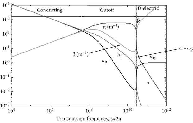
FIGURE 8.6
Plasma medium: conducting, cutoff, and dielectric regions.
8.4Plasma Medium
In Equation 8.22, we defined a new quantity ωp, called the angular plasma frequency, which is proportional to the square root of the electron density. In this section, we will explore the characteristics of the medium, called plasma medium. Plasma state is a fourth state of matter, the other three being solid, liquid, and gaseous states. On heating a solid material, we can successfully obtain liquid and gaseous states. If we heat the material further, we can obtain an ionized gas. The electrons are stripped away from the neutral atoms and in this state of matter we have positive ions and free electrons. Though the electrons are no longer bound in the atom, they are still subject to some restoring forces due to Coulomb forces between positive charges and negative charges. The effect of these long-range Coulomb forces, which vary as 1/r2, may be understood by considering the following one-dimensional problem. Consider a plasma medium that has positive ions and electrons with overall charge neutrality to begin with. As shown in Figure 8.7, let us assume that we disturbed the equilibrium situation by displacing a layer of electrons by a small distance z. At one end, there will be an excess of electric charge, −Nqz per unit area and at the other end, there will be an excess of positive ion charge +Nqz per unit area. The electric field created by this imbalance from charge neutrality at the ends may be calculated from the boundary condition Dn = ρs = Nqz. Hence,
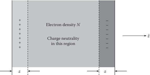
FIGURE 8.7
Oscillation of an electronic charge layer in a plasma medium.
The force experienced by an electron in the presence of this electric field is given by
Equating this to the inertial force, we can write the force balance equation as follows:
Equation 8.40 is an equation of oscillatory motion with the solution
where ω2p is given by Nq2/mε0. Thus, ωp gives the natural frequency of oscillation of the electronic charge layer.
8.5Polarizability of Dielectrics
If there are N molecules for unit volume, then the polarization may be written as
where αT is the molecular polarizability and g the ratio between local field Eloc acting on the molecule and the applied field E. These two fields differ because of the presence of surrounding molecules. Since εr = 1 + χe, we obtain from Equation 8.42,
It can be shown that
if the surrounding molecules act in a spherically symmetric fashion. Figure 8.8 shows the applied and local fields for the spherically symmetrical case.

FIGURE 8.8
Molecular polarizability and local field.
The polarization P=ˆzP creates equivalent charges on the walls. The equivalent charge dq on the walls is given by P · ds, where ds is the vector differential surface element on the sphere given by ˆrr20sinθdθdϕ. Therefore, the electric field dEp at the center of the sphere is given by
Since
and
From Equations 8.43 and 8.44, we obtain
This is called the Clausius–Mossotti relation. We have noted from the above equations that the local field is different from the applied electric field. However, in writing the force Equation 8.16, the RHS is electric force on the charge due to the applied electric force. If we use, instead, the force due to local electric field, then Equation 8.20 has to be modified: in Equation 8.20, replace ω0 by ω1, where
Figure 8.9 shows the general shape of εp versus ω1, where εp is given by Equation 8.21 with ω1 replacing ω0.
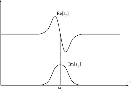
FIGURE 8.9
Dispersion and complex permittivity.
The complex permittivity
has analytical properties given by the Kramer–Kronig relations:
The polarization αT has contributions from several effects and may be written as
where the subscripts e, i, and d stand for electronic, ionic, and permanent dipole contributions to the polarizability, respectively. The electronic and ionic components may be generalized in the form
where Fj is the measure of the strength of the jth resonance. The permanent dipole contribution is different in the sense that the force opposing the complete alignment of the dipoles in the direction of the applied electric field is of thermal nature:
where T is the temperature, kB the Boltzmann constant, p the permanent dipole moment, and τ the relaxation time. Figure 8.10 [4] is a sketch of frequency response of a hypothetical dielectric.

FIGURE 8.10
Frequency response of a hypothetical dielectric.
In addition to the three polarization mechanisms discussed above, interfacial polarization or space–charge polarization [3] gives rise to a complex dielectric constant:
This polarization is due to the large-scale field distortions caused by the piling of space charges in the volume or of the surface charges at the interfaces between different small portions of materials with different characteristics. Geophysical media are examples [4] of such materials.
8.6Mixing Formula
Mixing formula gives the effective dielectric constant of dielectric inclusions of a material of dielectric constant εr2 embedded in a host dielectric material of dielectric constant εr1. Let the inclusions be spheres of radius a. Let the radius a be small when compared to the wavelength. This assumption permits us to ignore the effects of scattering. Let the spheres be sparsely distributed in the host material so that the fractional volume f, which is a fraction of the volume occupied by the spheres, is lower than a few percent, f ≪ 1. This assumption permits us to ignore the consideration of a correlation between spheres. The situation described here is similar to the situation described in Section 8.5, where the dielectric constant of the material consisting of many dipoles is given by
where N is the number of dipoles per unit volume and α the polarizability of the dipole. In our case, the effective dielectric constant εe is given by
where N is the number of spheres per unit volume. The polarizability α of the sphere is given by [3]
Equation 8.64 is obtained after making several simplifying assumptions, some of which are stated above.
Since
where V is the volume of the sphere, we obtain the effective dielectric constant as
In the above equation, we have
This is called the Maxwell–Garnet mixing formula. If the inclusion has a nonspherical shape, then the expression for α for that shape should be used. For more information on mixing formulas, see [3,5].
8.7Good Conductors and Semiconductors
The transport of charge gives rise to the flow of current, and the constitutive relation of a simple conductor is given by J = σE. Based on the magnitude of σ, we classify conductors into
semiconductors (σ ~10−2 S/m) and
conductors (metals and alloys) (σ ~10−2 − 108 S/m).
In general, the charge carriers in a conductor are free electrons, whereas in a semiconductor the charge carriers are electrons as well as holes. We have seen that σDC = Nq2/mν. We can use this expression for the conductivity σ provided ω < ν and ν2≪ω2p. These conditions are satisfied in metals for frequencies right up to optical frequencies. The conductivity of metals may also be written in terms of its electron mobility μe, where
The power dissipation per unit volume is
Let us discuss the collision frequency ν a little more in the context of conductors. The mean free path Λ of an electron can be related to the average drift velocity of the electron:
Here τ is the average collision time and is related to the collision frequency ν by
In the context of conductors, τ is also called relaxation time. Since the conductivity depends on the average collision time, the electrical resistivity ρ = 1/σ increases with temperature. It may be expressed in terms of its value ρRT at room temperature TR as
For pure metals, αR, the temperature coefficient of resistivity, is about 0.004/°C. For a table of values for αR, see [5]. As the absolute temperature T approaches zero, the pure metal has zero resistivity and becomes typically a superconductor. The temperature dependence of conductivity σ in pure metals as dictated by the mobility of electrons may be written as
Intrinsic semiconductors belong to group IV elements that include silicon and germanium. The conductivity of intrinsic semiconductors may be expressed as
where Nn and Np are the intrinsic electron and hole densities, respectively. Theoretical and experimental studies show that σ can be expressed in terms of forbidden gap energy Eg [5]:
Germanium (Ge) has a gap energy of 0.67 eV, while silicon (Si) has an Eg of 1.12 eV. Ge has a higher mobility than Si, hence Ge devices can be operated at higher frequencies. However, Ge devices are more sensitive to temperature changes. Extrinsic semiconductors are made by adding impurities (dopants) to the intrinsic semiconductors. The dopants are from group III or group V elements. The electrical properties of extrinsic semiconductors are strongly influenced by the dopants. N-type semiconductors have dopants, from group V (e.g., phosphorous) and have a set of easily activated electrons in the conduction band. Thus, donor impurities add to the free-electron population in the conduction band, facilitating an increased conductivity of the material. The P-type semiconductors are constituted by the addition of impurity atoms from group III elements (e.g., aluminum) and the impurity atoms are called acceptors. The conductivity of N-type is given by
where ND is the donor concentration. The conductivity of P-type is given by
where NA is the acceptor concentration.
Effective masses of electrons and holes in semiconductors are different from free electron mass due to various interactive force fields experienced by the charge carriers. As an example, for silicon, m*e/m0≈0.190−0.260 and m*h/m0=0.5, where m*e is the effective mass of the electron, m*h the effective mass of the hole, and m0 the mass of the free electron. For more details, see [5]. When a semiconductor is subjected to crossed electric (E) and magnetic (H) fields, a small potential field (EH) orthogonal to H and E is induced. This phenomenon is called the Hall effect and is discussed in Chapter 11.
8.8Perfect Conductors and Superconductors
The resistivity of many metals and alloys drops abruptly when they are cooled to a sufficiently low-temperature Tc (Figure 8.11a). The superconductivity state [5,67] is destroyed and normal conductivity state is restored if the current density Jc or the magnetic field Hc exceeds a threshold value. An empirical law relating Hc with the temperature T is given by [5]
where Hc0 is the critical magnetic field at T = 0. The boundary between superconductivity state and normal conducting state is shown in Figure 8.11b.
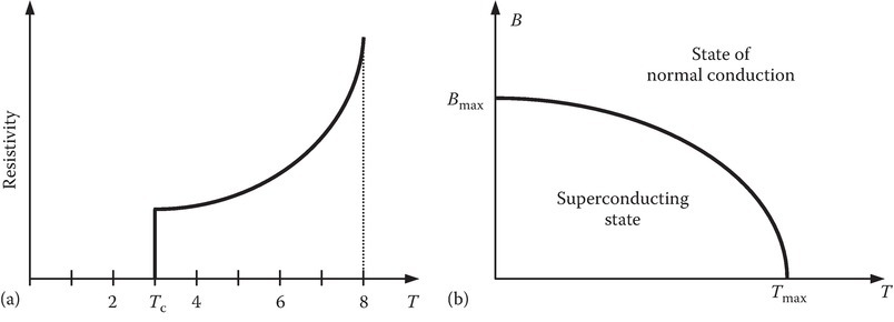
FIGURE 8.11
Superconductor: (a) resistivity versus temperature and (b) limits of Bmax and Tmax for superconducting state.
The empirical relation between Bmax and Tmax is given by
Provided that the current density, the magnetic field, and the temperature are less than the threshold values, the resistivity drops to zero and the conductor may be treated as a perfect conductor. As we noted in the previous section, a DC magnified field HDC can exist in a conductor even though EDC = 0. However, in a perfect superconductor, it will be shown that HDC = 0. Thus, a perfect superconductor is not only a perfect conductor, but also a perfect diamagnet. The magnetic field in a specimen is expelled as the temperature is brought below the critical temperature Tc. This phenomenon is called the Meissner effect. We investigate the electromagnetic phenomena in a superconductor based on a macroscopic theory given by London.
Instead of the usual Ohm’s law for normal conductors, that is,
London postulated that in a superconductor, the current density Js is given by
where C is a constant characteristic of a given material and A the usual vector potential. Taking the curl of Equation 8.81, we have
From Ampere’s law of direct current, we have
Since ∇ · B = 0,
The solution of Equation 8.86 for a semi-infinite superconductor occupying the space z > 0 is given by
where
and B is in x−y-plane. We will show later that
where ns is the density of superconducting electrons, and q and m are the charge and mass of an electron, respectively. Thus,
which is a real quantity. Equation 8.87 shows that λL is the length characterizing the decay of the flux density from its value at the surface of the superconductor. It is called the London penetration depth. For lead, λL = 146 Å. In a good normal conductor, the time-harmonic magnetic field penetrates to a depth δ:
where f is the frequency. For direct current, δ = ∞, signifying uniform distribution of DC magnetic field. In a superconductor, even for DC, λL is very small; this explains the Meissner effect. Let us next give a phenomenological basis for Equation 8.81. The current density Js in the superconductor is given by
where n*s is the density of carriers of charge qs and vs is their drift velocity. In the presence of a magnetic field Bs = ∇ × As, the total momentum Ps is
where ms is the mass of the charge carriers. The last term is the additional momentum due to the presence of the magnetic field. From Equations 8.92 and 8.93, we have
For super electrons, the total momentum is zero, provided
Equation 8.95 is obtained by making use of Equation 8.81. To calculate λL, we need to find the values to be used for ms, n*s, and qs. In a superconducting state, the electrons are loosely associated as pairs [6]. The electrons in a given pair have momentum ℏk and −ℏk, so that the net pair momentum is zero. The electron pair behaves like a single particle, giving rise to
where m, q, and ns are the mass, absolute value of the charge, and the number density of the electrons in a superconducting state, respectively. For a superconductor, the charge carriers are paired electrons. Substituting Equation 8.96, Equation 8.97 and Equation 8.98 into Equation 8.95, we see that Equation 8.95 is the same as Equation 8.89. From Equation 8.90, we see that λL should always be finite. Perfect superconductor, which is a perfect diamagnetic (Meissner effect of flux exclusion), is an idealization of a practical situation where λL ≪ l, where l is the relevant dimension of the sample.
A two-fluid model of superconductors at high frequencies is developed by considering that a fraction of the electrons are in superconductive state and they form pairs. In normal conductors, free electrons are assumed to move under the influence of the electric field and experience collisions as described earlier. The superconducting electron pairs, however, are immune from collisions. In the two-fluid model, we write separate momentum equations for each of the fluids, the normal fluid denoted by the subscript n and the superconducting fluid by the subscript s:
For a time-harmonic field, we have from Equations 8.99, 8.100, 8.102, and 8.103 that
where τ = 1/ν is the momentum relaxation time. An equivalent circuit for the above may easily be constructed as shown in Figure 8.12, where the analogy is

FIGURE 8.12
Circuit analogy for a superconductor based on the two-fluid model.
In the above circuit, V = jωLsIs and from the analogy
From the analogy of the second branch,
and
By comparison,
Note that for ω = 0, ωLn = 0, and Rn is short-circuited by ωLs. Thus, for T < Tc, although there are normal as well as superconducting electrons, the resistivity is identically zero. If ω is finite, then Rn is no longer shorted.
Maxwell’s equations for the superconductor, based on the two-fluid theory, are written as
The wave equation for H may be written as
Note that λL = ∞, if ns = 0. The last term on the LHS is negligible for a good conductor. This term arises because of the displacement current in the conductor. Let us obtain a one-dimensional time-harmonic solution, assuming
The magnetic field satisfies the equation
where δ=1/√πfμ0σn is the skin depth.
Assuming further
where
For the direct current case, δ = ∞, θ =1, and γ = 1/λL. λL is the penetration depth of HDC in a superconductor. This parameter is the quantitative measure of the Meissner effect. If it is a normal conductor and ω ≠ 0, then δ is finite, λL is large, and
thus
as expected.
The surface resistance may be calculated, following the steps in Section 2.5. Alternatively, for a unit width and unit length along y and x axes, respectively,
where
From Equations 8.135 and 8.136,
Since, E0 is the electric field on the surface at z = 0,
and from Maxwell’s equation 8.115,
Thus, we obtain the relation between E0 and H0:
The surface impedance is
8.9Magnetic Materials
Magnetic materials [4,5,6] get magnetized. The quantitative measure of magnetization is given by the magnetization vector M (A/m3), which is the net magnetic dipole moment pm per unit volume. It is analogous to the polarization P (C/m2), which is the net electric dipole moment per unit volume.
One can think of an analogous situation with reference to magnetic charges and define a magnetic dipole moment
where the magnetic charges +qm and −qm are separated by a small distance d. It is worth noting at this time that we cannot isolate magnetic charges, they can appear only as a pair, and the monopole magnetic charge density is zero. When we view currents as the sources of magnetic fields, we can draw the following analogy of a magnetic dipole and a loop of current (see Figure 8.13). At a greater distance, they have the same vector potential:
where
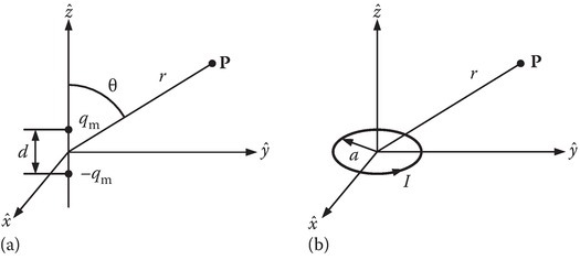
FIGURE 8.13
Equivalence of (a) magnetic dipole with a (b) small circular loop of current.
For a more general loop of current,
If the loop is planar and the origin is in the plane (Figure 8.14),
and
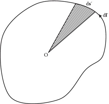
FIGURE 8.14
Planar loop.
If the source is a volume current J, then
The vector magnetic potential due to a volume of magnetic dipoles (Figure 8.15) of dipole density M (A/m) is given by
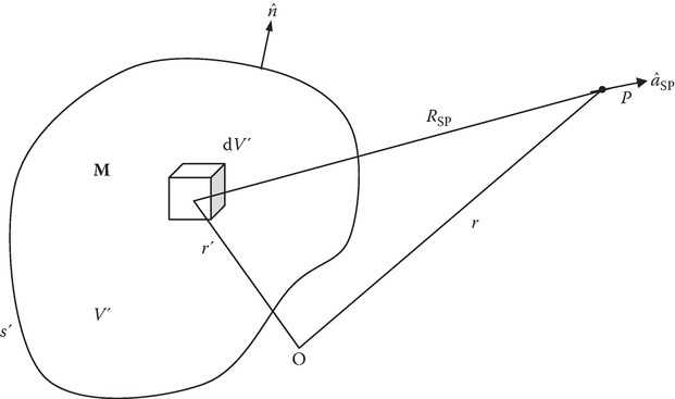
FIGURE 8.15
Volume of magnetic dipoles.
Equation 8.149 may be manipulated to yield
By comparing Equation 8.150 with the expressions for A due to volume current of density Jb and surface current of density Kb, the following equivalence may be given (Figure 8.16):
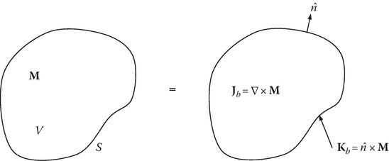
FIGURE 8.16
Equivalence of volume of magnetic dipoles with current distributions.
A topic of interest connected to a magnetic dipole is the torque T experienced by the dipole when it is brought into an external B field. It is given by
A current loop experiences a torque in the presence of an external B field. The loop will rotate and when the normal to the plane of the loop is parallel to B, an equilibrium is achieved. An electron in an orbit constitutes current. If an electron of charge −q executes an orbital motion of angular velocity ω, the corresponding current is given by
where ω depends on the environment to which the electron is subjected. Consider the simplest case of an electron circulating around a proton of charge +q in the presence of a magnetic field H0 perpendicular to the circular orbit (Figure 8.17).
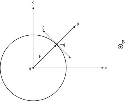
FIGURE 8.17
Electron circulating around a proton in the presence of a magnetic field perpendicular to the circular orbit.
From Lorentz force equation,
Assuming that the massive proton is stationary, we have
where we have used the relation v = ωr. The term mω2r on the RHS of the above equation is the counterbalancing centrifugal force due to the circular motion of the electron. Solving for ω,
where
In the above, ω0 is the frequency of circulation in the absence of H0. If ωL ≫ ω0, then corresponding to the case of large H0 or large r,
where ωL is called the Larmor frequency and ωb is called the cyclotron frequency. On the other hand, if H0 is small or r is small (ωL ≪ ω0), then the case for electrons orbiting in an atom is
Diamagnetic materials have μr slightly less than 1. It occurs in materials where the spin magnetization, explained later, is zero. The magnetization is only due to orbital motion. The magnetization due to the electrons spinning on their axis is zero due to even number of spins. The orbital magnetic dipole moment is given by
The net dipole moment per unit volume M that arises from the orbital motion of the electrons is opposite to the original H field and when related to the field through magnetic susceptibility χm,
where χm will be a negative value. This results in a relative permeability μr:
which is slightly less than 1. The above explanation is oversimplified but serves the purpose of showing that magnetization due to the orbital motion only leads to diamagnetization.
A simple explanation for paramagnetism in which μr is slightly larger than 1 is in terms of magnetization due to electron spin. The electrons of an atom with an even number of electrons usually exist in pairs, with the members of pairs having opposite spin directions, thereby canceling each other’s spin magnetic moment. If the number of electrons is odd, individual atoms have net magnetic moment. If an external magnetic field is applied, then the individual atoms will align with it subject to the randomizing effect of thermal motion. The magnetic moments partially line up with the external fields giving rise to positive susceptibility. However, in paramagnetic material, the coupling between the magnetic moments of various atoms is relatively weak.
Ferrimagnetic materials have magnetized domains. A magnetized domain of a material (of 10−10 m3 size) has atoms that are aligned parallel to each other (typically of the order of 1010 atoms in a domain). The domains are randomly oriented but in the presence of external fields they align. Examples of ferromagnetic materials are iron, nickel, and cobalt. The relative permeability is of the order of 3000. They exhibit nonlinearity, residual magnetism, and hysteresis. Soft ferromagnetic materials have narrow hysteresis loops and hence they can be more easily magnetized and demagnetized. Ferromagnetic materials are, in general, metallic in nature and their low resistivity gives rise to high eddy current losses at microwave frequencies. These losses are proportional to the square of the frequency and also proportional to the cube of the sample thickness. Laminating usually reduces these losses. At microwave frequencies, the losses are still large for vacuum-deposited thin ferromagnetic films of ~100–10,000 Å.
Ferromagnetic materials, known as ferrites and garnets, have high resistivity of up to 107 Ω m when compared to 10−7 Ω m for iron. This material is a mixture of metallic oxides of high resistivity. They have a lower magnetization and are not used in applications requiring high flux density as in power transformers. They are very useful at microwave frequencies. The high-resistivity property arises because, unlike ferromagnetic materials, the constituents of ferrite materials, both metallic and oxygen ions, have no free 3s or 4s electrons available for conduction. Ferrites in the presence of a static magnetic field behave as an anisotropic magnetic material. The wave propagation in such a material is discussed in Appendix 11B.
8.10Chiral Medium [8,9]
Figure 8.18 shows an approximation to a single turn left-handed and right-handed helix. The approximation consists of a circular conducting loop in a plane (x–y-plane) of radius a and a conductor of length 2l along the normal to the plane (z-axis). The distance between the turns (pitch) of the helix is 2l.

FIGURE 8.18
Approximate model for a helix: (a) left-handed and (b) right-handed.
Assume a time-harmonic incident electric excitation field E0 along the z-axis. The voltage induced is given by
The current is
where ZH is the impedance of the helix. The electric dipole moment due to electric excitation is
Note that for a time-harmonic field,
The magnetic dipole moment, due to electric excitation, in this case is
Next consider the case of time-harmonic magnetic excitation along the z-axis, ˆzH0. From Faraday’s law, we have
and the induced current I in the loop is given by
The magnetic dipole moment due to magnetic excitation is
The electric dipole moment due to magnetic excitation is
The point of the above calculation for the helix is to show that an electric excitation produces not only electric dipole moment, but also magnetic dipole moment. Since polarization is electric dipole moment per unit volume and magnetization is magnetic dipole moment per unit volume, we have shown that a material which has helices embedded in it experiences not only polarization, but also magnetization in the presence of an electric excitation. Similar remark can be made regarding magnetic excitation. Such a material is bi-isotropic in the sense that the constitutive relations are given by
where ε and μ are, respectively, the scalar permittivity and permeability of the media and ξc is the chirality admittance. The word chiral in Greek means handedness and chiral materials include elements having a handedness property. An artificial chiral medium may be constructed by embedding metal helices of one handedness in a host medium (Figure 8.19). Axes of the helices are randomly oriented to create an isotropic chiral medium.

FIGURE 8.19
Artificial chiral medium.
Bahr and Clansing [9] give the following details of an artificial chiral material.
Helices
n (helix density) = 20 × 106/m3,
a (radius of the helix) = 0.625 mm,
b (wire diameter) = 0.1524 mm,
2l (pitch of the helix) = 0.667 mm,
N (number of turns in a helix) = 3.
Nonchiral host material
Silicon rubber: constitutive parameters at 7 GHz,
μh = μ0 (1− j0),
εh = ε0 (2.95 − j0.07).
In the above μh and εh are, respectively, the permeability and permittivity of the host medium at the operating frequency. The constitutive relations for a chiral medium are given some times in the form of
In this notation, favored by Lindell–Sihvola [8], εc and μc are the effective permittivity and permeability of the chiral material, respectively, and κ is a scalar chiral parameter. The above-mentioned artificial chiral material has the following parameter values at f = 5 GHz:
Bahr and Clansing [9] have given the following results for κ as a function of frequency (Figure 8.20). The chirality parameter is negligible much below 5 GHz and also much above 10 GHz. This is understandable since the artificial medium has a length scale of cm.
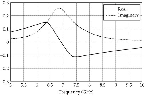
FIGURE 8.20
Chirality parameter κ versus frequency.
Example of a material that exhibits chiral properties at optical frequencies is sugar. Such a property arises since these molecules have an inherently helical character and the length scale is much shorter than the artificial medium mentioned above. A discussion of wave propagation in a chiral medium is given in Appendix 8A. Kalluri and Rao [10] discuss chiral filters. DeMartinis [11] discusses artificial chiral materials with conical inclusions.
8.11Plasmonics and Metamaterials
Plasmonics, a broad area of research in the subject of “Electromagnetics and Plasmas,” is having a resurgence of interest because of new applications [12,13]. Metamaterials are engineered artificial materials “with properties and functionalities not found in nature” [14], helping to remove or decrease some limitations of the devices constructed from purely natural materials. Of particular interest are those that have negative permittivity and negative permeability in some frequency bands. In such a frequency band, the material is called left-handed. This material is different from the chiral left-handed material discussed in the previous section. The qualifier ‘left-handed’ is used here in a different sense and is explained in Appendix 8B.
Much is claimed and expected from these materials. They are under intense investigations by many research groups. The Appendix 8B based on transmission line analogies of electromagnetic metamaterials [15] is a simple and short account to establish the connection with the transmission line theory.
References
- 1.Balanis, C.A., Advanced Engineering Electromagnetics, Wiley, New York, 1989.
- 2.Heald, M.A. and Wharton, C. B., Plasma Diagnostics with Microwaves, Wiley, New York, 1965.
- 3.Ishimaru, A., Electromagnetic Wave Propagation, Radiation and Scattering, Prentice Hall, Englewood Cliffs, NJ, 1991.
- 4.Ramo, S., Whinnery, J.R., and Van Duzer, T., Fields and Waves in Communication Electronics, Wiley, New York, 1994.
- 5.Neelakanta, P.S., Handbook of Electromagnetic Materials, CRC Press, Boca Raton, FL, 1995.
- 6.Soohoo, R.F., Microwave Magnetics, Harper & Row, New York, 1985.
- 7.Kadin, A.M., Introduction to Superconducting Circuits, Wiley, New York, 1999.
- 8.Lindell, I.V., Sihvola, A.H., Tretyakov, S. A., and Viitanen, A. J., Electromagnetic Waves in Chiral and Bi-Isotopic Media, Artech House, Boston, MA, 1994.
- 9.Bahr, A.J. and Clansing, K. R., An approximate model for artificial chiral material, IEEE Trans. Antennas Propag., AP-42, 1592, 1994.
- 10.Kalluri, D.K. and Rao, T. C. K., Filter characteristics of periodic chiral layers, Pure Appl. Opt., 3, 231, 1994.
- 11.DeMartinis, G., Chiral media using conical coil wire inclusions, Doctoral thesis, University of Massachusetts Lowell, Lowell, MA, 2008.
- 12.Maier, S.A., Plasmonics: Fundamentals and Applications, Springer, New York, 2007.
- 13.Veksler, D.B., Plasma wave electronic devices for THZ detection, Doctoral thesis, Rensselaer Polytechnic Institute, Troy, NY, 2007.
- 14.Noginov, M.A. and Podolskiy, V.A., Tutorials in Metamaterials, CRC Press, Taylor & Francis Group, Boca Raton, FL, 2012.
- 15.Caloz, C. and Itoh, T., Electromagnetic Metamaterials, Wiley, Hoboken, NJ, 2006.