
]>
Appendix 10A: Thin Film Reflection Properties of a Warm Isotropic Plasma Slab between Two Half-Space Dielectric Media*
10A.1Introduction
Thin metal films will play an important role in next-generation integrated optoelectronics. Exploiting photon–electron coupling and the propagation of electron–plasma waves (plasmonics) shows great promise in building nanosized sensors. Modeling the reflection properties of thin metal films integrated with dielectrics provides valuable insights into device response to waves in the optical spectrum in terms of frequency, film thickness, and angle of incidence. Optical imaging devices using surface plasmons, at nanometer scale resolution, are being fabricated that has enhanced photocurrent, responsivity, and bandwidth [1]. Thin-film gratings are being fabricated using complex nanoimprinting methods for next-generation lithographic technology, where dielectrics/ferroelectrics/metals are integrated into single substrates to build tunable surface plasmon resonance filters [2]. Thin films fabricated as photonic crystal back-reflectors with, enhanced optical absorption, have potential for light harvesting in high-efficiency solar cell applications [3]. Understanding the behavior of waves as they interact with metal/dielectric films is crucial for building novel sensing devices.
Within an order of magnitude of the plasma frequency of a metal, some interesting phenomena occur as oscillations of the power reflection coefficient caused by the internal interference of fields within the slab [4]. The nature of the oscillations, such as the frequency and amplitude are a function of the slab thickness, obliqueness of the incident wave, indices of refraction of the bounding materials, and the spatial dispersion of the metal itself. This chapter describes the physical model of the thin film and the behavior of the power reflection coefficient. The warm plasma model will be used based on the hydrodynamic approximation that will show oscillations in the power reflection coefficient. Based on film thickness, the effect of power tunneling caused by the interaction of evanescent waves will be shown in the region of total internal reflection.
The wave equation for a warm, compressible, anisotropic magnetoplasma was derived by Unz [5]. Prasad [6] derived the power reflection coefficient using state–space methods for a warm plasma slab in the free space and described the maxima/minima points as well as the characteristic roots q. Kalluri and Prasad [7] described the thin film reflection properties of a cold plasma slab in the free space for the isotropic case and described the oscillations internal to the slab where the maxima/minima were derived. The papers from Kalluri and Prasad consider nI = nT = 1. The power reflection coefficient in this chapter is derived from detailed equations starting from Maxwell’s equations and the hydrodynamic approximation with consideration of different input/output materials. The input transverse wave is obliquely incident on the slab interface, which reproduces itself inside the plasma, and, in addition, supporting longitudinal acoustic waves from the interface, with different wave numbers.
Special cases of the power reflection coefficient are presented for different refractive indices in frequency space. The overall power reflection coefficient is periodic with decreasing periodicity. When the acoustic mode velocity approaches zero, the plasma becomes cold and incompressible. The longitudinal characteristic roots are dependent on the parameter δ = a/c, where a is the acoustic velocity of the electron plasma wave. In certain metals the Fermi velocity [8] plays the role of the acoustic velocity. When a is comparable to c, that is, δ ≈ 0.1–0.01, the plasma is spatially dispersive and is considered to be warm. A small percentage change in the velocity of the longitudinal component gives rise to a dynamic response of the power reflection coefficient, of note, which is periodic with a slight aperiodicity. In addition, the oscillations within the warm plasma reflection coefficient tend to ride atop the cold plasma component.
10A.2Formulation of the Problem
To describe the electromagnetic waves inside the thin film, the metal is modeled as a lossy (collisions) homogeneous, isotropic (no static →B0

FIGURE 10A.1
Oblique incidence of a (TM or p) wave on a warm plasma slab and reflection/transmission waves. I, incident; R, reflected; T, transmitted; P, plasma.
A parallel (TM or p) wave EI is incident on the slab at an angle θI with reflected wave at angle θR = θI and transmitted wave at angle θT all on the plane of incidence.
10A.2.1Waves Outside the Slab
For the incident, reflected, and transmitted (I, R, and T) waves outside the plasma slab, the electric and magnetic fields obliquely incident can be described as
where →EI,R,T0 and →HI,R,T0 are the complex electric and magnetic amplitudes given by
ψI,R,T is the phase reference of the waveform at →r=0,
From Figure 10A.1, the geometry of the wave vector can be described as
where ST = kI/kTS and CT=√1−(kI/kTS)2. ST and CT describe the characteristics of the dielectric in the output of the system. Note, S = sin(θI), C = cos(θI), ST = sin(θT), and CT = cos(θT). If kI = kT, then ST = S and CT = C. Since the position vector is →r=ˆxx+ˆyy+ˆzz, the phase factor of the waves outside the plasma slab become
where C′=√(kT/kI)2−S2=(kTkI)CT. From ψT, k2T,x+k2T,z=k2T, where kTω/c√εT=ω/cnT=k0nT. The angle-dependent parameter, C′, in ψT (Equation 10A.5) was derived using Snell’s law. Snell’s law implies that the boundary conditions (or phase match) has been satisfied as is evident in the x-component of (Equation 10A.5) and also by the fact that θI = θR. The x-components of the phase factor for the incident, reflected, and transmitted waves are the same to satisfy the boundary conditions, and hence, for the TM wave the tangential components of →E and →H are continuous across the boundary in both space and time.
For a plane wave propagation [9], the electric and magnetic fields can be described as
where μ0 is the free-space permeability. Using Equation 10A.1 in Equation 10A.6, we obtain
where ηI = η0/nI.
10A.2.2Waves Inside the Slab
The basic equations for a warm plasma are Maxwell’s equations:
Using the hydrodynamic approximation for a compressible electron gas the conservation of momentum [5] (isotropic case)
The conservation of energy is
The equation of state is
where N, N0 are the small and large signal number density (m−3), p, p0 the small and large signal pressure (kg/m s2), T, T0 the small and large signal temperature (K), °K the Boltzman constant, γ the specific heat in constant pressure/specific heat in constant volume, m the electron mass (kg), →u the velocity vector (m/s).
The formulation given above is based on the linear theory. Unz showed that Equations 10A.8 and 10A.9 reduce to the wave equation
where
and Z is described in terms of the electron collision frequency ν and transmission frequency ω:
The term
is inversely proportional to the normalized frequency squared, X = 1/Ω2, where Ω = ω/ωp. Within the film four modes exist: Transmitted/reflected transverse waves and transmitted/reflected longitudinal waves. The boundary at z = 0, d serves to act as the source of an acoustic wave mode only supported within the slab medium. Within the slab, a TM wave and an acoustic wave with velocity, pressure, and electric field intensity, both satisfy the wave equation (10A.10). In this chapter, the dimensionless parameter np can be described in terms of the input medium, input angle, and plasma characteristic root parameter, q′:
where q′ will be determined. Note: q′ is not the derivative of q but rather distinguishes between a nI > 1 dependent solution of the dispersion equation and a nI = 1 solution. For a warm plasma, the velocity of the longitudinal component is significant and in certain metals is approximately two to three orders of magnitude less of the speed of light c. The electric and magnetic field intensities inside the plasma can be described as
The electric and magnetic fields in Equation 10A.15 have complex field amplitudes as
The phase of the fields within the plasma slab is defined as
When using Equations 10A.15 and 10A.16 in Equation 10A.10, one has for oblique incidence on the slab interface:
Equation 10A.18a, Equation 10A.18b and Equation 10A.18c can be rearranged in a matrix form as
which is
The components of Equation 10A.20 come from Equation 10A.18a, Equation 10A.18b and Equation 10A.18c and are as follows:
Setting determinant of [F] to zero yields the dispersion relation F11F33 − F13F31 = 0. The characteristic roots for the cold and warm plasma models are derived directly from the dispersion relation
Subscript 1 indicates an upward-going wave and subscript 2 indicates a reflected downward-going wave of the transverse type, similarly the subscripts 3 and 4 of the longitudinal type. Using Equation 10A.8 to find the magnetic field intensity yields
Since the incident wave is a TM wave, only the y-component matters, and hence
From dispersion relation and Equation 10A.24, the ratio of the magnetic to electric tangential components becomes
The warm plasma electric field-dependent electron velocity field is given by
where β0 = eN0/jωε0 = ωmX/je. Using Equations 10A.21a and 10A.21c, Equation 10A.26 becomes
10A.2.3Power Reflection Coefficient for a Warm Isotropic Plasma Slab between Two Different Dielectric Media (i.e., nI and nT)
In considering the case where the plasma medium is warm, a longitudinal electric field must be taken into account. The power reflection coefficient is derived for a warm plasma sandwiched between two different dielectric media nI and nT. Using Equations 10A.25 and 10A.27 with the following equations for a collisionless plasma, U = 1, we have
We use boundary conditions where the tangential components of →E and →H are continuous at z = 0 and d to generate four equations. For time-harmonic waves, tangential boundary conditions are used as they are derived by Maxwell’s curl equations. Normal boundary conditions (from divergence equations) can be derived from the curl equations. Hence, normal boundary conditions are not independent but are assured to be satisfied when the tangential boundary conditions are satisfied [10]. Two more equations are generated from the boundary conditions to account for the z component of the electron velocity to be zero at the interfaces since there is no electron flow within the dielectrics. Writing the system of equations from the boundary conditions, Equation 10A.1, Equation 10A.2, Equation 10A.3, Equation 10A.4, Equation 10A.5, Equation 10A.6 and Equation 10A.7 and (10A.28):
The longitudinal component of the waveform inside the plasma is comprised of the electric field only, since ηy3 is equal to zero. Putting Equation 10A.29 in a matrix form gives
where λ′i=e−jk0nIq′id,ET′x=ETxe−jk0nIC′d,andHT′y=HTye−jk0nIC′d.
The complex reflection coefficient can be solved by the ratio of the reflected and incident electric fields
The symbol ‖ implies that the incident and reflected waves are p-waves on the plane of incidence. After substantial simplification of Equation 10A.31, ‖R‖ becomes
where
The power reflection coefficient is defined by the magnitude squared of ‖R‖
A closed form of Equation 10A.34 is not given here because of its high complexity; it can either be studied using computer code or from approximation. The refractive indices nI and nT cause the angle-dependent parameter C′ to become zero at the critical angle. The real and imaginary parts of the complex reflection coefficient change depending on whether the incident angle is less than or greater than the critical angle. Equation 10A.34 is much dependent on nI and nT such that the choice of material will dramatically change the reflection properties of the composite material. Figure 10A.2 shows the power reflection coefficient for a normalized film thickness of dp = d/λp = 0.2, where λp is the plasma wavelength, λp = 2πc/ωp, an input angle of θI = 60° and materials nI = 1.1 and nT = 1.3 with δ = 0.1. The power reflection coefficient changes from a monotonic to a complex oscillatory behavior that occurs between zero and one with a periodicity that decreases with increasing frequency.
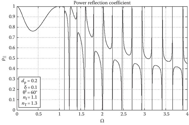
FIGURE 10A.2
Power reflection coefficient for dP = 0.2, δ = 0.1, θI = 60°, nI = 1.1, and nT = 1.3.
10A.3Different Regions of the Power Reflection Coefficient
A method in understanding the reflection properties is by examining that the dispersion relation, when solved, leads to the characteristic roots of the plasma medium. For the isotropic case, there are four roots in total, two for an upward- and downward-going set of transverse modes, q′1,2 and similarly two for a set of longitudinal (acoustic) modes, q′3,4. The transverse modes can be considered as the cold plasma modes and the longitudinal modes can be considered as the warm plasma modes. For the lossless case U = 1, the characteristic roots will be either real or imaginary but not complex. The zeros of the roots, considered here as critical points, are dependent on a number of parameters. The critical points are also the points where the roots change from real to imaginary and vice versa. Equation 10A.22 shows that as Ω approaches zero the characteristic roots approaches infinity. In addition, as Ω approaches infinity, the roots asymptotically reach levels dependent on the incident angle. The critical points divide ρ‖ into three main regions (see Figure 10A.3): The first region, 0 < Ω < [1 − (δnIS)2]−1/2: both q′1 and q′3 are imaginary causing total reflection of the incident power for thick materials. Note, in ρ‖ there is another phenomenon known as power tunneling that will be described to explain a dip seen in this first region for thin materials. The first region is also where attenuated total reflection (ATR) can occur by careful choice of index material and incident angle. The second region [1 − (δnIS)2]−1/2 < Ω < [1 − (nIS)2]−1/2: q′1 is still imaginary but q′3 is real allowing the longitudinal (acoustic) plasma wave to propagate through the plasma. In this region, ρ‖ takes on an oscillatory behavior as a result of the internal reflections of the longitudinal component. For the case of nI = nT = 1, an approximation to ρ‖ is made to show that the oscillatory behavior is from the longitudinal mode only. Deriving a cosecant term that determines the zeros ρ‖ (approximate) shows a q′3 only dependence. The frequency of the oscillations can change dramatically with small changes in film thickness indicating a large sensitivity of the film properties. The third region, [1 − (nIS)2]−1/2 < Ω < ∞: both q′1 and q′3 are real and the transverse and longitudinal waves are propagating through the slab. Oscillations of a different complexity occur in ρ‖ for this third region.
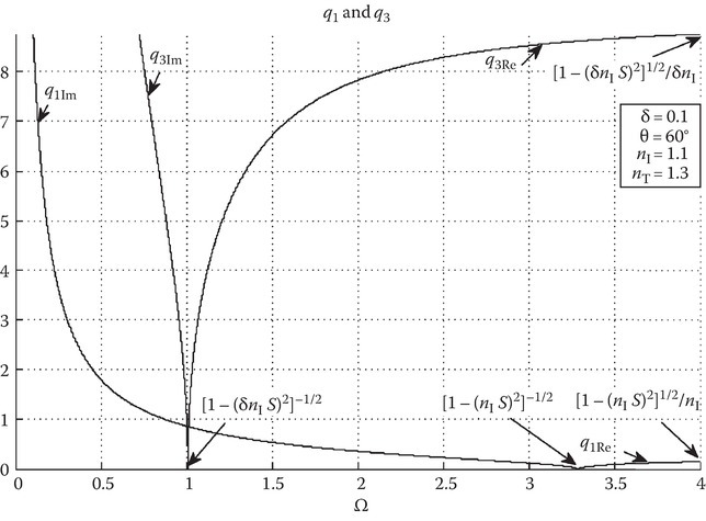
FIGURE 10A.3
Characteristic roots for δ = 0.1 and θ = 60°. The critical points are shown for refractive index nI = 1.1. Both q′1 and q′3 do not depend on nT.
Varying the incident angle or material properties nI can dramatically change the zeros of q′1 and q′3 (see Figure 10A.3). This sets the critical points for ρ‖ which changes its dynamic. The critical points bound the regions of ρ‖ and can be described as
The following sections describe in detail the behavior of ρ‖ within the regions bounded by the critical points of q′. Equation 10A.32 is analyzed for a few special cases.
10A.3.1Power Reflection Coefficient for Region 1, 0 < Ω < [1 − (δnIS)2]−1/2
Based on Figure 10A.3, the respective characteristic roots are
All of the λ′i terms will be real, and hence, Equation 10A.32 will consist of hyperbolic sines and hyperbolic cosines only. As a result, there is no propagation of either transverse or longitudinal modes and the waves are evanescent. The power reflection coefficient will have no oscillations and will stay at unity for this region. The following section will show that as the film gets sufficiently thin, power tunneling will take effect and ρ‖ will not always be unity, but will allow some power to propagate, or tunnel, through the slab.
10A.3.1.1Region 1 and the Effects of Power Tunneling
For thick slabs, the waves are evanescent and the decaying fields will not interact. When the slab becomes sufficiently thin power tunneling will occur. The tunneling represents itself as a peak in region 1 of the transmission coefficient τ‖. Kalluri [11] gave an expression at the peak which is a transcendental equation related to the phase term of oscillation in ρ‖. Tuning Ω and measuring the peak in τ‖ for a known incident angle gives Ωmax that can lead to determining the slab thickness or the plasma frequency.
Figure 10A.4 shows the effect of power tunneling for normalized thicknesses of dp = 0.05, 0.1, 0.2, 1, and nI = nT = 1. The power transmission coefficient, τ‖ = 1 − ρ‖, is also shown. For thin films at λp/20, the slab is almost completely transmissive. For dP = 1, the intensity of light impinging on the warm plasma slab is completely reflected away from the interface. However, as the thickness of the slab decreases, the cross-interaction between evanescent forward-going electric and backward-going magnetic (and vice versa) fields create a real propagating power in a plane parallel to the interface that emerges at z = d. This explains the dip seen in this first region. For the air–plasma–air cold plasma case, an experimental measurement of the maximum power transfer could yield information about the material thickness with the use of a transcendental equation. As the thickness of the slab increases, this phenomenon decreases as the decaying fields within the slab become negligibly small as they reach the opposite interface. Figure 10A.5 shows results for dielectric–plasma–dielectric cold and warm plasma case, nI = 1.46, nT = 1.48. For all thicknesses, there is a noticeable difference in the tunneling effect between the cold plasma model (δ = 0) and the warm plasma case (δ = 0.1) and there are differences when different dielectrics are introduced.
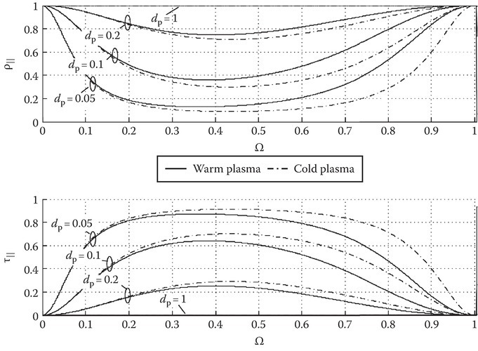
FIGURE 10A.4
Region 1, 0 < Ω < [1 − (δnI S)2]−1/2. This shows the power reflection coefficient at different film thickness: dp = 0.05, 0.1, 0.2, and 1. Refractive indices are nI = nT = 1 and the warm plasma plots have δ = 0.1 with θ = 60°. The bottom plot is the transmission coefficient, τ‖ = 1 − ρ‖.
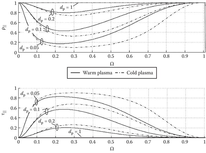
FIGURE 10A.5
Region 1, 0 < Ω < [1 − (δnI S)2]−1/2. Similar to Figure 10A.4 but with nI = 1.46, nT = 1.48.
Looking at both Figures 10A.4 and 10A.5, the largest difference between warm and cold is seen in ρ‖ at dp = 0.05 near the plasma frequency. For all thicknesses, more light transmits through the slab for the cold plasma model. In the measurement of optical constants, the dip seen for 0 ≤ Ω ≤ 1 can provide valuable information about the material np with knowledge of nI and nT by an appropriate correction factor to the transcendental equation. In addition, the figures show that at Ω = 0, 1, ρ‖ = 1. From Equation 10A.32 as Ω → 0 (ω = 0), X → ∞ then as shown in Figure 10A.3, q1 → ∞ and q3 → ∞. Subsequently, ηy1, βz1 → 0, βz3, λ′i→∞ and ‖R‖ → 1. When Ω = 1 (ω = ωp), then X → 1, ηy1 → 0, βz1, βz3 → −1 and λ′i will all be equal, then ‖R‖ → 1. For both Ω = 0, 1, ρ‖ is forced to unity, independent of any nI or nT creating a confluence point for any choice of material.
10A.3.1.2Region 1 and Surface Plasmons
If one considers the electron plasma wave velocity a to become several orders of magnitudes slower than c = 3 × 10⁸ m/s, then from Equations 10A.22 and 10A.28b, δ → 0, q3 → ∞, βz3 → ∞ and the plasma is cold. Also, from Equation 10A.32, only the terms multiplied by β2z3 survive and one can derive the power reflection coefficient for a cold plasma between two different dielectrics,
Plotting Equation 10A.37, Figure 10A.6, using the material chosen by Lekner [12] and Otto [13] the input dielectric was glass of nI = 1.9018, silver film of np = 0.055 + j3.28, which is based on the plasma frequency, and lithium fluoride of nT = 1.392 as the output medium. Collisions were taken into account as is indicated by the real part of np.

FIGURE 10A.6
The power reflection coefficient at two different film thicknesses versus angle of incidence in degrees: d = 35 and 55 nm. Refractive indices are nI = 1.9018, nT = 1.392, and np = 0.055 + j3.28.
The result in Figure 10A.6 compares quite well with Lekner’s result. From the results of Equation 10A.37, the collision term of np causes a nonzero real part of q′. Since this is the case of ATR, the frequency corresponding to the wavelength of λ = 546.1 nm is below the plasma frequency and in the region of total reflection. Figure 10A.6 also shows the C′ term, which can be shown to be zero at the critical angle C′=√(nT/nI)2−S2(θ=47.05°)=0 causing ρ‖ to transition downward to zero as photons couple to electrons exciting a surface plasmon at the surface plasmon angle of 53.9°. The critical angle (47.05° for this case) is the point where C′ turns from a purely real number to a purely imaginary number. This zero point is the angle at which total internal reflection would occur and the wave would travel along the boundary if no film was present between nI and nT. The critical angle is also the point where the analytical expressions for the real and imaginary parts of ‖R‖ (not shown in this chapter) change, hence, Re{∥R∥}θI<θC≠Re{∥R∥}θI>θC and Im{∥R∥}θI<θC≠Im{∥R∥}θI>θC. The surface plasmon resonance is the effect of a metal film present sandwiched between nI and nT. In a sense, the insertion of the metal film induces an equivalent Brewster angle for an incident p-wave that would not exist for the half-space materials only. From Averitt [14], the angle where the power reflection coefficient is totally suppressed, and for the real part of εP the surface plasmon resonance can be calculated as
10A.3.2Power Reflection Coefficient for Region 2, [1 − (δnIS)2]−1/2 Ω < [1 − (nIS)2]−1/2
Based on Figure 10A.3, the respective characteristic roots are
The power reflection coefficient takes on an oscillatory dynamic. The purely real q3 implies that the longitudinal (acoustic) mode will propagate through the film. The λ′i terms in Equation 10A.32 containing q3 will be complex implying propagation of power through the slab. As can be seen in Figure 10A.2, the oscillations in this region are dramatic as a result of the spatially dispersive plasma medium. The warm plasma component is an acoustic mode of electrostatic field intensity with amplitude and velocity a, it is longitudinal, and is a solution to Maxwell’s equations. When a is small compared to c, there is no wave propagation and the plasma becomes cold, then only plasma oscillations exist at ωp. The λ′i terms containing q1 will be real and the transverse modes will be evanescent.
10A.3.2.1Region 2 and an Approximation of ρ‖ for nI = nT = 1
Since, sin(k0jq1d) ≡ j sinh(k0q1d) and cos(k0jq1d) ≡ cosh(k0q1d),
The power reflection coefficient in this region can be approximated and put into a simpler form and can be written as
where
The A2 term does not contribute much to Equation 10A.41 when compared to A3 and A4. The A3 and A4 terms are large and negative for most of the region of interest, as such, A2 can be neglected. An approximation to Equation 10A.41 (designated as ρa) becomes
which can be reduced to
Equation 10A.44 is in the same form as the cold plasma slab result reported by Kalluri and Prasad [7]. The plots for ρ‖ and ρa are given in Figure 10A.7 for δ = 0.3 with film thickness of dp = 1. Region 2 is approximately {1.04 < Ω < 2}. The approximation of ρ‖ is very good until Ω ≈ 1.86. Values of Ω in the region ~1.86 < Ω < 2 is where A2 ≈ A3 ≈ A4 and the suppression of the A2 term is no longer valid in Equation 10A.43. The oscillations have a periodicity that decreases as Ω increases, which is caused by the Ω-dependent csc2 term. Although there is an oscillatory term in the bracketed term [sin( )]2, the zeros of ρa are not determined by this term but are completely dependent on the phase of the csc2 term, and hence
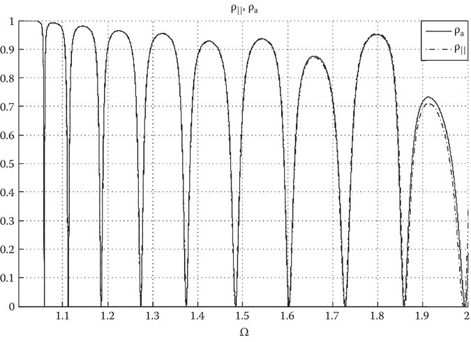
FIGURE 10A.7
Comparison of Equations 10A.40 and 10A.44 and their approximation. Refractive indices are nI = nT = 1, δ = 0.3, input incident angle of θ = 60°, and film thickness is dp = 1.
At m = 0,1,2, …, the csc2 term goes to infinity defining discrete zeros for ρa and consequently for ρ‖. The peaks seen in Figure 10A.7 are at values of Ω where dρa/dΩ = 0. If one allows Equation 10A.44 to become
where A5 = A0(q1q3 sin(k0q3d) + S2X sinh(k0q1d)) and A6 = k0q3d + tan−1(−A4/A3) ± π/2.
Then from Equation 10A.46, the equation to find the peaks of ρa is a transcendental equation,
where
and
10A.3.2.2Region 2 and Film Thickness
Figure 10A.8 shows ρ‖ (Equation 10A.34) for different slab thicknesses dp = 0.05, 0.1, 0.2, 0.5, 0.7, and 1. The index of refraction of the dielectrics are nI = nT = 1, with δ = 0.1 and an input incident angle of θ = 60°. The range for this region is 1.0037 < Ω < 2. As the thickness increases, the number of oscillations increases. The amplitude of the oscillations spans the entire range between zero and one. Since nI = nT = 1, the points where ρ‖ = 1 are when q1q3 sin(k0q3d) = −S2X sinh(k0q1d). The points where ρ‖ = 0 are when the phase of the csc2 is equal to mπ.
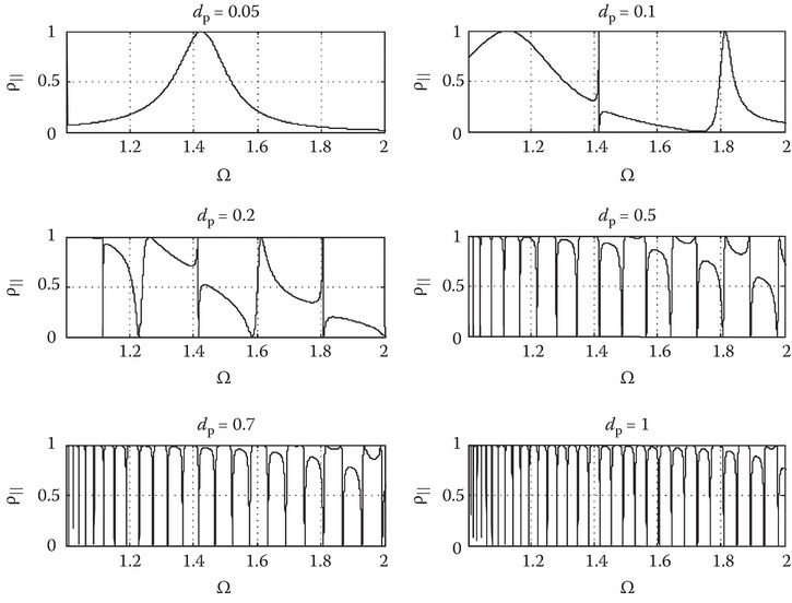
FIGURE 10A.8
Plots of the power reflection coefficient for different film thicknesses. Refractive indices are nI = nT = 1, δ = 0.1, input incident angle of θ = 60°, and film thicknesses of dp = 0.05, 0.1, 0.2, 0.5, 0.7, and 1.
For the case where nI = 1.4, nT = 1.45, the range of Ω has no second critical point, and hence 1.0074 < Ω < j1.458. This implies that q′1 stays imaginary for all Ω as shown in Figure 10A.9. The refractive indices for the input and output mediums have the effect of tuning the second critical point of q′1 which changes the behavior of the oscillations in ρ‖. Shown in Figure 10A.10, as the thickness increases, sharp notches in the frequency band occur.

FIGURE 10A.9
q′1 and q′3 for nI = 1.4, nT = 1.45 in the frequency range of 1.0074 < Ω < ∞.
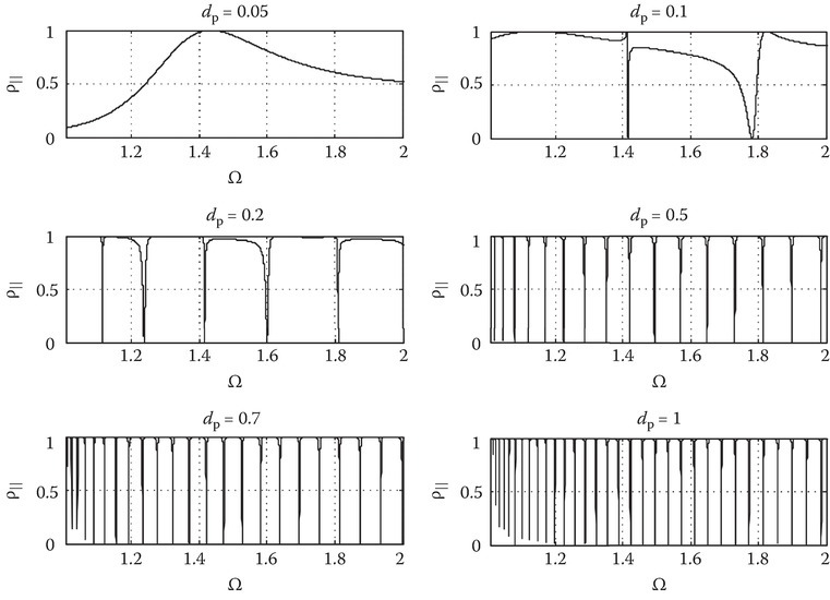
FIGURE 10A.10
Plots of the power reflection coefficient for different film thicknesses. Refractive indices are nI = 1.4, nT = 1.45, δ = 0.1, input incident angle of θ = 60°, and film thicknesses of dp = 0.05, 0.1, 0.2, 0.5, 0.7, and 1.
Power Reflection Coefficient for ([1 − (nIS)2]−1/2 < Ω < ∞). Region 3, where both q′1 and q′3 are real will be discussed in a future paper.
10A.3.3Power Reflection Coefficient for a Sodium Thin Film
Using the material properties of Na from Forstmann and Gerhardts [8]: The plasma frequency is ωp = 8.2 × 10¹⁵ rad/s, with a Fermi velocity of VF = 9.87 × 107 cm/s resulting in δ = VF/c = 3.29 × 10⁻³. Using a film thickness of d = 10 nm and an incident angle of θ = 60°, Figure 10A.11 shows the power reflection coefficient for the warm (top) and cold (bottom) plasma model. Only the first two regions are shown since the third region is unbounded based on the input and output materials. The first region (0 < Ω < 1) shows the effect of power tunneling as seen as the large dip. The plasma wavelength of λp = 229 nm is large when compared with the 10 nm film thickness. The oscillations in the second region are very clear as a result of the Fermi velocity of the metal film. The warm plasma oscillations ride atop of the cold plasma result. Similar to previous results, the periodicity of the oscillations caused by real q3 and imaginary q1 decrease as the Ω increases.

FIGURE 10A.11
Plots of the warm and cold power reflection coefficients for a sodium (Na) material thin film with thickness of d = 10 nm. Refractive indices are nI = 1.45, nT = 1.46, the plasma frequency for sodium is ωp = 8.2 × 10¹⁵ rad/s, and the Fermi velocity is VF = 9.87 × 107 cm/s resulting in δ = VF/c = 3.29 × 10⁻³. The input incident angle is θ = 60°. Power reflection coefficient (a) δ = 0.00329, and (b) δ = 0.
10A.4Conclusion
Reflection properties for a thin metal slab bounded by two different dielectrics have been presented with emphasis on the power reflection coefficient and its corresponding characteristic roots. The film was modeled as a warm plasma that supports a longitudinal electromagnetic acoustic mode that is a solution to Maxwell’s equations. The oscillations in the power reflection coefficient follow the trend of the cold plasma component. The cold plasma case was presented for different dielectric materials and the model shows surface plasmon excitation.
The choice of the material has an impact on the characteristics of the energy propagating through the plasma material. The characteristic roots are dependent on the index of refraction of the input material, the velocity of the longitudinal plasma wave, and the angle of incidence.
Choice of the refractive index of the input material such that nIS = 1, makes q1 purely imaginary for all frequencies. The sines and cosines, which are functions of q1 wave number become hyperbolic, creating power reflection coefficient similar to comb function of slightly decreasing periodicity. Hence, the refractive index of the input medium has the effect of tuning the reflection properties of the thin film.
Markos and Kalluri [15] have recently published an updated version of the material in this chapter.
References
- 1.Shackleford, J. A., Grote, R., Currie, M., Spanier, J. E., and Nabet, B., Integrated plasmonic lens photodetector, Appl. Phys. Lett., 94, 083501-1–083501-3, 2009.
- 2.Chen, H. L., Hsieh, K. C., Lin, C. H., and Chen, S. H., Using direct nanoimprinting of ferroelectric films to prepare devices exhibiting bi-directionally tunable surface plasmon resonances, Nanotechnology, 19, 1–6, 435304, 2008.
- 3.Curtin, B., Biswas, R., and Dalal, V., Photonic crystal based back reflectors for light management and enhanced absorption in amorphous silicon solar cells, Appl. Phys. Lett., 95, 083501-1–083501-3, 231102, 2009.
- 4.Stratton, J. A., Electromagnetic Theory, IEEE Press, Piscataway, NJ, p. 513, 2007.
- 5.Unz, H., Oblique wave propagation in a compressible general magnetoplasma, Appl. Sci. Res., 16, 105–120, 1965.
- 6.Prasad, R. C., Transient and frequency response of a bounded plasma, PhD thesis, Birla Institute of Technology, Ranchi, India, 1976.
- 7.Kalluri, D. K. and Prasad, R. C., Thin-film reflection properties of isotropic and uniaxial plasma slabs, Appl. Sci. Res., 27, 415–424, 1973.
- 8.Forstmann, F. and Gerhardts, R. R., Metal Optics near the Plasma Frequency, Springer, Berlin, Germany, pp. 9–24, 1986.
- 9.Pozar, D. M., Microwave Engineering, Wiley, New York, pp. 21–24, 1998.
- 10.Ramo, S., Whinnery, J. R., and Van Duzer, T., Fields and Waves in Communication Electronics, 3rd edition, Wiley, New York, p. 147, 1994.
- 11.Kalluri, D. K., Electromagnetics of Time Varying Complex Media: Frequency and Polarization Transformer, 2nd edition, CRC Press, New York, pp. 26–27, 2010.
- 12.Lekner, J., Theory of Reflection, Developments in Electromagnetic Theory and Applications, Academic Publishers, Dordrecht, the Netherlands, pp. 169–170, 1987.
- 13.Otto, A., Spectroscopy of surface polaritons by attenuated total reflection, in: Seraphin, B. O. (Ed.), Optical Properties of Solids: New Developments, North-Holland, Amsterdam, the Netherlands, p. 703, 1976.
- 14.Averitt, R. D., Plasmonics and metamaterials at terahertz and mid-infrared frequencies, IEEE LEOS Plasmonics Workshop, MIT Lincoln Laboratory, Lexington, MA, October 30, 2007.
- 15.Markos, C. T. and Kalluri, D., Thin film reflection properties of a warm isotropic plasma slab between two half-space dielectric media, J. Infrared Millim. Terahertz Waves, 32, 914–934, 2011.