
]>
6
Laplace Equation: Static and Low-Frequency Approximations*
In an ideal transmission line, the voltage phasor ˜V
where
The time-harmonic equation in three dimensions (Helmholtz equation) is given by
where
and ∇2 is the Laplacian operator.
If the frequency is zero (f = 0) or low such that β2 = k2 ≈ 0, the Helmholtz equation can be approximated by the Laplace equation.
Static or low-frequency problems satisfy the Laplace equation
where Φ is called the potential. In the first undergraduate course in electromagnetics, the one-dimensional solution of the Laplace equation in various coordinate systems is discussed and illustrated through simple examples. In the following section, we list these solutions for completeness.
6.1One-Dimensional Solutions
Cartesian coordinates:
Cylindrical coordinates:
Spherical coordinates:
6.2Two-Dimensional Solutions
6.2.1Cartesian Coordinates
In Chapter 3, we solved the waveguide problem by solving the Helmholtz equation
by assuming
where f1(x) and f2(y) are given in the form of a template, given, respectively, by Equations 3.15 and 3.16, where k2c=k2x+k2y.
The implication is that if one of the first four elements in Equation 3.15 is chosen for the x-variation, then one of the last four elements in Equation 3.16 has to be chosen for the y-variation, and |kx| = |Ky|. The choice of f1(x) and f2(y) can be reversed, if the boundary conditions require such a choice. The point is illustrated through an example.
Example 6.1: Figure 6.1 shows the geometry for the example.
Let the boundary conditions be
Solution
From B.C.1 and B.C.2, the y-variation is
From B.C.3, the x-variation has to be
B.C.4 is satisfied if n = 3. Thus,
From B.C.4,
A little thought would show that we could have written the solution (Equation 6.9) by inspection. The factor sinh(3πa/b) in the denominator neutralizes the value of sinh(3πx/b), when x = a is substituted in the process of implementing B.C.4. The constant 100 is the Fourier coefficient of the third harmonic. B.C.4 requires only the third harmonic of the Fourier series. All other Fourier coefficients are zero if we considered the expansion of f(y) = 100 sin(3πy/b) in Fourier series. Suppose f(y) is a more general function than given in B.C.4. Obviously, the Fourier coefficients of other harmonic can be nonzero and
Let us illustrate such Fourier series solution through Example 6.2.
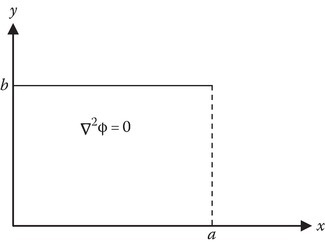
FIGURE 6.1
Geometry for Example 6.1.
Example 6.2: Same as Example 6.1, except that
Solution
The boundary at x = a is a conductor of constant voltage of 100 V.
We have to determine the Fourier coefficient Bn when f(y) is defined to be a constant in the interval 0 < y < b (Figure 6.2).
We will make two interesting points about the Fourier expansion being sought in this problem. The Fourier series is for a periodic function. However, the function f(y) is only defined over half of the period of the fundamental sin(πy/b). The full period of the fundamental is 2b. Since the desired Fourier series is to have only sine terms, the function has to be an odd function. The function can be continued for the full period, from (−b) to (+b), as shown in Figure 6.3.
Note that the solution is valid only in the field region 0 < x < a and 0 < y < b; the continuation of f(y) in the region beyond 0 < y < b, is immaterial to the validity of the solution in the field region; however, the condition is important in determining the Fourier coefficients [1].
For the problem on hand,
Since f(y) is an odd function of y and sin(nπy/b) is an odd function of y, the product is an even function and evaluating for the given f(y):
Thus,
Example 6.2 brings out several interesting points.
The boundary conditions 1, 2, and 3 dictated the type of the restricted Fourier series expansion, in the example sine series only, and the continuation of the periodic function, beyond the original domain, can be constructed to achieve the restricted Fourier series. In Appendix 6A, we examine the possible periodic continuation of a function x(t), defined over a finite range 0 < t < t1, so that the Fourier series will have
odd harmonic only;
sine terms only (Example 6.2);
cosine and odd harmonic only;
sine and odd harmonic only.
In subsequent sections, we will be discussing the expansion of an arbitrary function defined over a finite interval in Bessel series and other orthonormal functions.
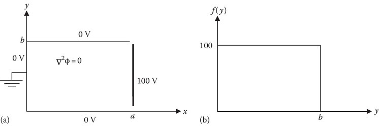
FIGURE 6.2
(a) Geometry for Example 6.2 and (b) function f( y) in B.C.4.

FIGURE 6.3
Periodic continuation of f (y) of Example 6.2 for having only sine terms in the Fourier series expansion.

FIGURE 6.4
Geometry for Example 6.3.
Example 6.3: Determine the potential in the field region described by the geometry given in Figure 6.4.
Solution
Let us write the solution for the problem by inspection, based on the experience we gained in solving Examples 6.1 and 6.2:
The steps that allowed us to write this solution by inspection are as follows.
Step 1: The requirement of multiple zeros on the x-axis including a zero at x = 0 leads to the choice of
Step 2: Since Φ = 0 when y = b, we choose
Note that sinh(mπ/a)(b − y) is a linear combination of sinh(mπy/a) and cosh(mπy/a), which are in the template of functions for f2(y).
Step 3: The term sinh(mπb/a) in the denominator is the neutralizing (normalizing) factor in satisfying the boundary condition Φ = 100, when y = 0, so that Bm = 400/mπ is the Fourier coefficient.
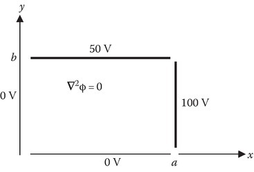
FIGURE 6.5
Geometry for Example 6.4.
Example 6.4: Determine the potential in the field region described in the geometry of Figure 6.5.
Solution
Example 6.4 is solved by using superposition (Figure 6.6).

FIGURE 6.6
The use of superposition for Example 6.4.
In Chapter 3, we simply studied the various modes that can exist in a waveguide with a view to get the cutoff frequencies of various modes. We did not study the excitation of the various modes by a source in a waveguide. The amplitudes of the various modes can be obtained by expanding the source function in the various modes. The modes often are the orthonormal functions permitting such expansions. Reference 2 makes use of such expansions.
6.2.2Circular Cylindrical Coordinates
Case 1:
Let us first consider that the potential is a function of the ρ and ϕ coordinates. Then
Let
Multiplying the above equation by ρ2/(f(ρ)g(ϕ)), we obtain
Term 1 is entirely a function of ρ and term 2 is entirely a function of ϕ, and hence each must be a constant and the sum of the constants must be zero. Denoting the separation constant by n2, Equation 6.23 can be written as two ordinary differential equations:
The solution for f(ρ) can be written as a linear combination of ρn and ρ− n and thus

FIGURE 6.7
Geometry for Example 6.5.
Example 6.5: Commutator problem
Figure 6.7 gives the geometry for the commutator problem. The field region is 0 < ρ < a and the upper part of the long cylinder is at the potential V0 and the bottom part is at the potential –V0.
Solution
From the physics of the problem, we know that the potential is finite at ρ = 0. The second term in the template for f(ρ), ρ−n, blows up as ρ tends to zero. Hence, we choose ρn as the ρ-variation. The boundary condition Φ (a, ϕ) = F(ϕ), sketched in Figure 6.8, is an odd function of ϕ.
So, by inspection, we write
and
Case 2:
Using the separation of variable technique, two ordinary differential equations can be obtained, in terms of the separation constant k2:
Equation 6.30 is the same as that of Equation 3.59 with n = 0. Therefore, the solution can be written as
or
where

FIGURE 6.8
Sketch of the function F(ϕ) for Example 6.5.
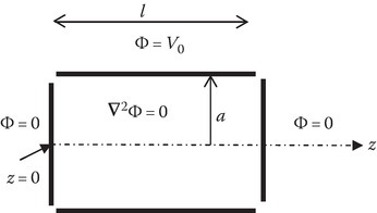
FIGURE 6.9
Geometry for Example 6.6.
Example 6.6: In the field region 0 < ρ < a and 0 < z < l, 0 < ϕ < 2π, the Laplace equation is satisfied.
The curved surface, ρ = a, 0 < z < l, is at a constant potential V0 as shown in Figure 6.9. The ends of the can are grounded.
Determine Φ(ρ, ϕ, z).
Solution
Note the symmetry with respect to the ϕ-coordinate and hence
Since we need multiple zeros on the z-axis and the potential is zero for z = 0, we choose
From Equation 6.33, noting K0 blows up when ρ → 0, we choose I0 for ρ variation and write by inspection
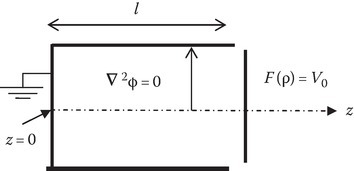
FIGURE 6.10
Geometry for Example 6.7.
Example 6.7: The field region is the same as that of Example 6.6. However, the boundary conditions are different and are shown in Figure 6.10:
The boundary condition Φ (a,z) = 0 requires an oscillatory function for ρ-variation. Hence, we choose, the template of Equation 6.32. Moreover, f1 has to be finite on the z-axis (ρ = 0). By inspection, we write
where pm = xom is the mth root of J0. A few of these values are given in Table 2.4.
The boundary condition Φ (ρ, l) = F (ρ) = V0 can be satisfied if
Equation 6.43 is an expansion of an arbitrary function in a Bessel series. Such an expansion, analogous to the Fourier series in trigonometric functions, is possible since these Bessel functions also possess orthogonal properties:
Multiplying Equation 6.43 by ρJ0(pqρ/a) and integrating from 0 to a, we obtain
Thus,
When F(ρ) = V0
Using the integral
we obtain
Substituting Equation 6.49 into Equation 6.47, we obtain
6.3Three-Dimensional Solution
6.3.1Cartesian Coordinates
The three-dimensional solution of the Laplace equation in a closed box may be obtained on the same line as the two-dimensional solution discussed in Section 6.2.1. One can also view the solution from the viewpoint of the rectangular cavity problem discussed in Section 4.1. The central point is that in the case of the Laplace equation,
which in turn means that if f1(x) and f2(y) are trigonometric functions, then f3(z) necessarily has to be the hyperbolic type. Example 6.8 illustrates the technique.
Example 6.8
In a rectangular box of dimensions a, b, and h, shown in Figure 4.1, the faces x = 0, a; y = 0, b; z = 0 are all at zero potential. For the face z = h, the potential is V0. Determine the potential Φ inside the field region 0 < x < a, 0 < y < b, and 0 < z < h.
Assume that the Laplace equation is satisfied in the field region.
Solution
The solution can be written by inspection as
Bmn is the Fourier coefficient of a double Fourier series expansion of the function
It can easily be evaluated using the orthogonality property and is given by
6.3.2Cylindrical Coordinates
Instead of trigonometric and hyperbolic functions, the template contains the Bessel functions and the modified Bessel functions for the ρ-variation.
6.3.3Spherical Coordinates
By substituting k = 0 in Equation 5.10, the equation for f1 can be obtained. Its solution gives
The equations for f2 and f3 are unchanged and are given, respectively, by Equations 5.11 and 5.13, and thus the three-dimensional solution of the Laplace equation in spherical coordinates is given by
The properties of the Legendre polynomials are given in Chapter 5.
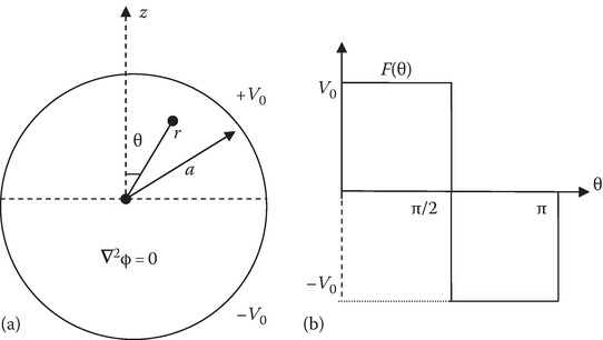
FIGURE 6.11
(a) Geometry and (b) sketch of the boundary condition for Example 6.9.
Example 6.9
In a spherical volume of radius a, the Laplace equation is satisfied. The top-half of the surface at r = a, 0 < θ < π/2, is at the voltage V0 and the bottom-half of the surface at r = a, π/2 < θ < π, is at –V0, as shown in Figure 6.11. Determine the potential inside and outside the sphere.
Solution
The boundary condition can be stated as
which is sketched in Figure 6.11b.
From the symmetry, it is obvious that the potential does not depend on the ϕ-coordinate. Thus, it is a two-dimensional problem. By choosing f3 = cos mϕ and m = 0, the ϕ dependence is removed:
Note that the associated Legendre polynomials of zero degree (m = 0) P0n or Q0n are called Legendre polynomials Pn or Qn, respectively. Figure 5.1 presents the graphs of these functions. Table 5.3 consists of the polynomial expressions, in terms of cos θ, of these functions.
For Example 6.9, the solution can be obtained separately for inside and outside the sphere.
Case 1: r < a.
From the boundary condition,
The coefficient An can be determined based on the orthogonality property listed in Table 5.3. Multiplying both sides by Pm sin θ and integrating, we have
Thus,
Substituting for f(θ), we obtain
Evaluating,
The solution is completed by evaluating other Am coefficients.
Case 2: r > a.
Example 6.10
This example [1] allows us to determine the field’s off-axis, knowing the fields on the axis of a circular loop. Consider the direct current in a circular loop of radius a, in the x–y-plane with the center of the loop at the origin. It is well known that the magnetic field at a point on the z-axis is given by
From the binomial expansion,
Thus, for z < a,
In a region where there are no currents, we have
where Φm is called the scalar magnetic potential and since
First consider r < a:
Note Pn|cos 0 = 1.
Comparing Equation 6.70 with Equation 6.64, we obtain
Thus,
There are several homework problems illustrating the use of the solution in spherical coordinates for practical static problems.
References
- 1.Ramo, S., Whinnery, J.R., and Van Duzer, T. V., Fields and Waves in Communication Electronics, 3rd edn., Wiley, New York, 1994.
- 2.Ji, C., Approximate analytical techniques in the study of quadruple-ridged waveguide (QRW) and its modifications, Doctoral thesis, University of Massachusetts Lowell, Lowell, MA, 2007.