Appendix 7A: Two- and Three-Dimensional Green’s Functions

Search in book...
Toggle Font Controls
Create new playlist

Name your new playlist

Playlist description (optional)
Sign In

Email address

Password

Forgot Password?

or

Continue with Facebook

Continue with Google
Sign Up

Full Name

Email address

Confirm Email Address

Password

or

Continue with Facebook

Continue with Google

7A.1Introduction

We discussed Green’s function briefly (Section 7.2). The one-dimensional Green’s function of the Laplace equation, with Dirichlet boundary conditions, is the solution of the differential equation

(7A.1a)

d 2 G d x 2 = - δ (x - x'), 0 < x < L,

$\frac{d^{2} G}{d x^{2}} = - δ (x - x^{'}), 0 < x < L,$

subject to the boundary conditions

(7A.1b)

G = 0, x = 0,

$G = 0, x = 0,$

(7A.1c)

G = 0, x = L,

$G = 0, x = L,$

and is shown to be

(7A.2a)

G = G 1 = x L - x ' L, 0 < x < x',

$G = G_{1} = x \frac{L - x^{'}}{L}, 0 < x < x^{'},$

(7A.2b)

G = G 2 = x ' ( L - x ) L, x' < x < L .

$G = G_{2} = \frac{x^{'} (L - x)}{L}, x^{'} < x < L .$

For an arbitrary input f(x), the response y(x) can be obtained from a superposition integral

(7A.3)

y (x) = \int 0 L f (x') G (x, x') d x' .

$y (x) = \int_{0}^{L} f (x^{'}) G (x, x^{'}) d x^{'} .$

The differential equation for y is

(7A.4a)

d 2 y d x 2 = - f (x), 0 < x < L,

$\frac{d^{2} y}{d x^{2}} = - f (x), 0 < x < L,$

and the boundary conditions are

(7A.4b)

y = 0, x = 0,

$y = 0, x = 0,$

(7A.4c)

y = 0, x = L .

$y = 0, x = L .$

Equation 7A.3 for y is the solution to Equation 7A.4, where G is given by Equation 7A.2. Equation 7A.3 may be written more explicitly, by considering the solution in the two domains 0 ≤ x ≤ x′ and x′ ≤ x ≤ L:

(7A.5a)

y (x) = \int 0 L x ( L - x ' ) L f (x') d x', 0 \leq x \leq x',

$y (x) = \int_{0}^{L} \frac{x (L - x^{'})}{L} f (x^{'}) d x^{'}, 0 \leq x \leq x^{'},$

(7A.5b)

y (x) = \int 0 L x ' ( L - x ) L f (x') d x', x' \leq x \leq L .

$y (x) = \int_{0}^{L} \frac{x^{'} (L - x)}{L} f (x^{'}) d x^{'}, x^{'} \leq x \leq L .$

Note: Some books define the Green’s function using a positive impulse for the input strength:

(7A.6)

d 2 G d x 2 = δ (x - x') .

$\frac{d^{2} G}{d x^{2}} = δ (x - x^{'}) .$

Then the solution will be of opposite sign to Equations 7A.2a and 7A.2b:

(7A.7a)

G = G 1 = x x ' - L L, 0 < x < x',

$G = G_{1} = x \frac{x^{'} - L}{L}, 0 < x < x^{'},$

(7A.7b)

G = G 2 = x' x - L L, x' < x < L .

$G = G_{2} = x^{'} \frac{x - L}{L}, x^{'} < x < L .$

We also considered the one-dimensional Helmholtz equation, with Dirichlet boundary conditions,

(7A.8a)

d 2 G d x 2 + k 2 G = - δ (x - x'),

$\frac{d^{2} G}{d x^{2}} + k^{2} G = - δ (x - x^{'}),$

(7A.8b)

G = 0, x = 0,

$G = 0, x = 0,$

(7A.8c)

G = 0, x = L,

$G = 0, x = L,$

(7A.9a)

G = G 1 = 1 k sin k x sin k ( L - x ' ) sin k L, 0 < x < x',

$G = G_{1} = \frac{1}{k} \frac{sin k x sin k (L - x^{'})}{sin k L}, 0 < x < x^{'},$

(7A.9b)

G = G 2 = 1 k sin k x ' sin k ( L - x ) sin k L, x' < x < L .

$G = G_{2} = \frac{1}{k} \frac{sin k x^{'} sin k (L - x)}{sin k L}, x^{'} < x < L .$

7A.2Alternate Form: Infinite Series

The procedure used in Section 7.2 is to solve the homogeneous equation in the two domains excluding the point x = x′ where the impulse is applied. Using the boundary conditions, and the source conditions, the undetermined constants were determined. The result is Green’s function in closed form. An alternative form will now be determined using eigenfunction expansion.

Let us solve Equation 7A.6 using this technique. The solution will be written as an infinite series

(7A.10)

G (x, x') = \sum n = 1 \infty a n (x') sin n π x L .

$G (x, x^{'}) = \sum_{n = 1}^{\infty} a_{n} (x^{'}) sin \frac{n π x}{L} .$

Note that each of the terms on the RHS of Equation 7A.10 satisfies the boundary conditions of G = 0 at x = 0 or L. From Equation 7A.10, we obtain

(7A.11)

d 2 G d x 2 = \sum (- n π L) 2 a n (x') sin n π x L .

$\frac{d^{2} G}{d x^{2}} = \sum {(- \frac{n π}{L})}^{2} a_{n} (x^{'}) sin \frac{n π x}{L} .$

By substituting Equation 7A.11 into Equation 7A.6, multiplying by sin mπx/L, and then integrating from 0 to L, we obtain

(7A.12)

- \sum (n π L) 2 a n (x') \int 0 L sin n π x L sin m π x L d x = \int 0 L δ (x - x') sin m π x L d x .

$\begin{matrix} - \sum {(\frac{n π}{L})}^{2} a_{n} (x^{'}) \int_{0}^{L} sin \frac{n π x}{L} sin \frac{m π x}{L} d x \\ = \int_{0}^{L} δ (x - x^{'}) sin \frac{m π x}{L} d x . \end{matrix}$

From the orthogonality property,

(7A.13)

\int 0 L sin n π x L sin m π x L d x = = 0, m \neq n L 2, m = n .

$\begin{matrix} \int_{0}^{L} sin \frac{n π x}{L} sin \frac{m π x}{L} d x & = & 0, m \neq n \\ = & \frac{L}{2}, m = n . \end{matrix}$

Thus, from Equation 7A.12, we get

- (m π L) 2 a m (x') L 2 a m (x') = = sin m π x ' L, - 2 L m 2 π 2 sin m π x ' L .

$\begin{matrix} - {(\frac{m π}{L})}^{2} a_{m} (x^{'}) \frac{L}{2} & = & sin \frac{m π x^{'}}{L}, \\ a_{m} (x^{'}) & = & - \frac{2 L}{m^{2} π^{2}} sin \frac{m π x^{'}}{L} . \end{matrix}$

Thus, we have

(7A.14)

G (x, x') = - 2 L π 2 \sum n = 1 \infty 1 n 2 sin n π x ' L sin n π x L .

$G (x, x^{'}) = - \frac{2 L}{π^{2}} \sum_{n = 1}^{\infty} \frac{1}{n^{2}} sin \frac{n π x^{'}}{L} sin \frac{n π x}{L} .$

Equation 7A.14 is an alternative form to Equations 7A.7a and 7A.7b, although Equation 7A.14 appears as an infinite series. The solution of

(7A.15)

d 2 y d x 2 = f (x)

$\frac{d^{2} y}{d x^{2}} = f (x)$

can be written as

(7A.16)

y (x) = - 2 L π 2 \sum n = 1 \infty 1 n 2 sin n π x L \int 0 L sin n π x ' L f (x') d x' .

$y (x) = - \frac{2 L}{π^{2}} \sum_{n = 1}^{\infty} \frac{1}{n^{2}} sin \frac{n π x}{L} \int_{0}^{L} sin \frac{n π x^{'}}{L} f (x^{'}) d x^{'} .$

The solution converges due to the term 1/n² in Equation 7A.16.

7A.3Sturm–Liouville Operator

A generalization of the series method for a one-dimensional problem with a general second-order differential equation is formulated in terms of a Sturm–Liouville operator L:

(7A.17a)

$[L + λ r (x)] y = f (x),$

where

(7A.17b)

$L = \{\frac{d}{d x} [p (x) \frac{d}{d x}] - q (x)\} .$

Let ψ_n be a complete set of orthonormal eigenfunctions for the L operator, that is,

(7A.18)

$[L + λ_{n} r (x)] Ψ_{n} (x) = 0$

subject to the same boundary condition as the original problem of Equation 7A.17a. If G(x, x′) is Green’s function

(7A.19)

$[L + λ r (x)] G (x, x^{'}) = δ (x - x^{'})$

subject to the same boundary condition as the original problem, then

(7A.20)

$G (x, x^{'}) = \sum_{n} \frac{Ψ_{n} (x^{'}) Ψ_{n} (x)}{λ - λ_{n}} .$

We will show two examples [1] of series form of Green’s function for two particular problems obtained from Equation 7A.20.

Example 1

(7A.6)

$\frac{d^{2} G}{d x^{2}} = δ (x - x^{'}) .$

Equation 7A.6 is a particular case of Equation 7A.19 where

$λ = 0, p (x) = 1, q (x) = 0, r (x) = 1, L = \frac{d^{2}}{d x^{2}} .$

The eigenfunctions are obtained from

$(L + λ_{n} r (x)) ψ (x) = [\frac{d^{2}}{d x^{2}} + λ_{n}] ψ_{n} = 0$

subject to the boundary conditions

$ψ_{n} = 0, x = 0 or L .$

Thus,

$\begin{matrix} ψ_{n} & = & \sqrt{\frac{2}{L}} sin \frac{n π x}{L} (orthonormal), n = 1, 2, \dots, \infty, \\ λ_{n} & = & {(\frac{n π}{L})}^{2}, \\ G (x, x^{'}) & = & \sum_{n} \frac{\sqrt{\frac{2}{L}} sin \frac{n π x^{'}}{L} \sqrt{\frac{2}{L}} sin \frac{n π x}{L}}{0 - {(\frac{n π}{L})}^{2}}, \end{matrix}$

which is the same as Equation 7A.14. The second example is Green’s function of Helmholtz equation (in series form)

Example 2

(7A.21a)

$\frac{d^{2} G}{d x^{2}} + β^{2} G = δ (x - x^{'}),$

(7A.21b)

$G (0) = G (L) = 0.$

Equation 7A.21a is a particular case of Equation 7A.19, where

$λ = β^{2}, p (x) = 1, q (x) = 0, r (x) = 1, L = \frac{d^{2}}{d x^{2}} .$

The orthonormal equations are

$\begin{matrix} ψ_{n} & = & \sqrt{\frac{2}{L}} sin β_{n} x = \sqrt{\frac{2}{L}} sin \frac{n π x}{L}, \\ λ_{n} & = & β_{n}^{2} = {(\frac{n π}{L})}^{2} . \end{matrix}$

Hence,

(7A.22)

$G (x, x^{'}) = \frac{2}{L} \sum_{n = 1, 2, \dots}^{\infty} \frac{sin (n π x^{'} / L) sin n π x / L}{β^{2} - {(n π / L)}^{2}} .$

To complete this section, here we will write down Green’s function in closed form for the Sturm–Liouville problem:

(7A.23a)

$G_{1} = G (x, x^{'}) = \frac{h_{2} (x^{'}) h_{1} (x)}{p (x^{'}) w (x^{'})}, 0 < x < x^{'},$

(7A.23b)

$G_{2} = G (x, x^{'}) = \frac{h_{1} (x^{'}) h_{2} (x)}{p (x^{'}) w (x^{'})}, x^{'} < x < L,$

where h₁(x) is the solution form of the homogeneous equation, in the interval 0 < x < x′, and h₂(x) is the solution form of the homogeneous equation, in the interval x′ < x < a:

(7A.23c)

$G_{1} (x) = A_{1} h_{1} (x),$

(7A.23d)

$G_{2} (x) = A_{2} h_{2} (x),$

and w(x′) is the Wronskian of h₁ and h₂ at x = x′:

(7A.23e)

$w (x^{'}) = h_{1} (x^{'}) h_{2}^{'} (x^{'}) - h_{2} (x^{'}) h_{1}^{'} (x^{'}) .$

The closed solution of Green’s function given in Equation 7A.9a and 7A.9b can be obtained from the general solution given in (7A.23) by noting

$p (x) = 1, h_{1} (x) = sin k x, h_{2} (x) = sin k (L - x)$

and the Wronskian w(x′) is obtained as

$\begin{matrix} w (x^{'}) & = & h_{1} (x^{'}) h_{2}^{'} (x^{'}) - h_{2} (x^{'}) h_{1}^{'} (x^{'}) \\ = & (sin k x) (- k) cos k (L - x) - sin k (L - x) (k) cos k x \\ = & - [sin k x cos k (L - x) + cos k x sin k (L - x)] \\ = & - [sin k (x + L - x)] \\ = & - k sin k L, \end{matrix}$

(7A.24a)

$G = G_{1} = \frac{sin k (L - x^{'}) sin k x}{- k sin k L}, 0 < x < x^{'},$

(7A.24b)

$G = G_{2} = \frac{sin k x^{'} sin k (L - x)}{- k sin k L}, x^{'} < x < L .$

The difference in sign between Equations 7A.24 and 7A.9 is because Equation 7A.9 is the response when the impulse is of strength −1.

7A.4Two-Dimensional Green’s Function in Rectangular Coordinates

7A.4.1Laplace Equation: Formulation and Closed Form Solution

(7A.25a)

$\frac{d^{2} G}{d x^{2}} + \frac{d^{2} G}{d y^{2}} = δ (x - x^{'}) δ (y - y^{'}),$

(7A.25b)

$\begin{matrix} x = 0 or a, G = 0, \\ y = 0 or b, G = 0. \end{matrix}$

Let us first write

(7A.26)

$G (x, y, x^{'}, y^{'}) = \sum_{n = 1, 2, \dots}^{\infty} g_{m} (y, x^{'}, y^{'}) sin \frac{m π x}{a} .$

Here, we formulated such that the boundary conditions at the walls x = 0 or a are satisfied.

By substituting Equation 7A.26 into Equation 7A.25a, we obtain

(7A.27)

$\begin{matrix} \sum_{m = 1}^{\infty} [- {(\frac{m π}{a})}^{2} g_{m} (y; x^{'}, y^{'}) sin \frac{m π x}{a} + sin \frac{m π x}{a} \frac{d^{2} g_{m} (y; x^{'}, y^{'})}{d y^{2}}] \\ = δ (x - x^{'}) δ (y - y^{'}) . \end{matrix}$

Multiply both sides of Equation 7A.27 by sin nπx/a and integrate with respect to x from 0 to a.

From orthogonality property, the LHS is

$\frac{a}{2} [- {(\frac{n π}{a})}^{2} g_{n} (y; x^{'}, y^{'}) + \frac{d^{2}}{d y^{2}} g_{n} (y; x^{'}, y^{'})]$

and the RHS is

$\int_{0}^{a} δ (x - x^{'}) δ (y - y^{'}) sin \frac{n π x}{a} d x = sin \frac{n π x^{'}}{a} δ (y - y^{'}) .$

Thus, the differential equation in y is obtained as

(7A.28)

$\frac{d^{2}}{d y^{2}} g_{m} (y; x^{'}, y^{'}) - {(\frac{m π}{a})}^{2} g_{m} (y; x^{'}, y^{'}) = \frac{a}{2} sin \frac{m π x^{'}}{a} δ (y - y^{'}) .$

Equation 7A.28 can now be solved by using the recipe of Equations 7A.23a and 7A.23b.

The homogeneous form of Equation 7A.28 is

(7A.29)

$\frac{d^{2} g_{m}}{d y^{2}} (y; x^{'}, y^{'}) - {(\frac{m π}{a})}^{2} g_{m} (y; x^{'}, y^{'}) = 0$

subject to the boundary condition g_m = 0, y = 0 or b (Figure 7A.1):

(7A.30a)

$A_{1} h_{1} (x) \to A_{m} h_{m}^{(1)} (y) = A_{m} (x^{'}, y^{'}) sinh \frac{m π y}{a}, region 1, 0 < y < y^{'},$

(7A.30b)

$A_{2} h_{2} (x) \to B_{m} h_{m}^{(2)} (y) = B_{m} (x^{'}, y^{'}) sinh \frac{m π (b - y)}{a}, region 2, y^{'} < y < b .$

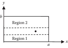
FIGURE 7A.1
Two-dimensional rectangular area divided into two regions: region 1, 0 < y < y′ − ε; region 2, y′ + ε < y < b.

Now the Wronskian from Equation 7A.23e, after simplification, becomes

(7A.30c)

$w (y; x^{'}, y^{'}) = - \frac{m π}{a} sinh \frac{m π b}{a} .$

From Equation 7A.23a, we obtain

(7A.31a)

$\begin{matrix} g_{m}^{(1)} (y; x^{'}, y^{'}) & = & \frac{(2 / a) \sin (m π x^{'} / a) ({h_{m}^{(2)} |}_{y^{'}}) ({h_{m}^{(1)} |}_{y})}{- (m π / a) \sinh (m π b / a)} \\ = & \frac{- (2 / m π) \sin (m π x^{'} / a) \sinh (m π / a) (b - y^{'}) \sinh (m π y / b)}{\sinh (m π b / a)}, 0 < y < y^{'} \end{matrix}$

From Equation 7A.23b, we obtain

(7A.31b)

$g_{m}^{(2)} (y; x^{'}, y^{'}) = \frac{- (2 / m π) sin (m π y^{'} / a) sinh [(m π / a) (b - y)]}{sinh (m π b / a)}, y^{'} < y < b .$

Now the complete Green’s function is given as

(7A.32a)

$\begin{matrix} G (x, y; x^{'}, y^{'}) & = & - \frac{2}{π} \sum_{m = 1}^{\infty} \frac{sin (m π x^{'} / a) sinh [(m π / a) (b - y)]}{m sinh (m π b / a)} \\ \times sin \frac{m π x}{a} sinh \frac{m π y}{a}, for 0 \leq x \leq a, 0 \leq y \leq y^{'} . \end{matrix}$

(7A.32b)

$\begin{matrix} = - \frac{2}{π} \sum_{m = 1}^{\infty} \frac{sin (m π x / a) sinh [(m π / a) (b - y)]}{m sinh (m π b / a)} \\ \times sin \frac{m π x^{'}}{a} sinh \frac{m π y^{'}}{a} for 0 \leq x \leq a, y^{'} \leq y \leq b . \end{matrix}$

We can develop an alternative form of Green’s function by first satisfying the boundary conditions at the walls y = 0 or b, that is, instead of Equation 7A.2 start with

(7A.33)

$G (x, y; x^{'}, y^{'}) = \sum_{n = 1, 2, \dots}^{\infty} g_{n} (x; x^{'}, y^{'}) sin \frac{n π y}{b}$

and develop the solution. The result is given in Equations 14.83a and b of Balanis [1].

7A.4.2Laplace Equation: Series Form (Bilateral) Solution

For series solution of Green’s function, we need the orthonormal eigenfunction ψ_mn for this two-dimensional problem.

These are the solutions of (for Laplace equation)

(7A.34a)

$\frac{\partial^{2} ψ_{m n}}{\partial x^{2}} + \frac{\partial^{2} ψ_{m n}}{\partial y^{2}} + λ_{m n} ψ_{m n} = 0$

subject to boundary condition

(7A.34b)

$\begin{matrix} ψ_{m n} & = & 0, x = 0 or a, \\ = & 0, y = 0 or b . \end{matrix}$

Of course, we know that the orthogonal eigenfunctions that satisfy the boundary conditions (Equation 7A.34b) are

$ψ_{m n} = A_{m n} sin \frac{m π x}{a} sin \frac{n π y}{b} .$

From orthogonality property,

$1 = \int_{x = 0}^{a} \int_{y = 0}^{b} {(ψ_{m n})}^{2} d x d y = \frac{a b}{4} A_{m n}^{2} .$

Thus, $A_{m n} = 2 / \sqrt{a b}$ ,

(7A.35a)

$ψ_{m n} = \frac{2}{\sqrt{a b}} sin \frac{m π x}{a} sin \frac{n π y}{b},$

(7A.35b)

$λ_{m n} = {[{(\frac{m π}{a})}^{2} + {(\frac{n π}{b})}^{2}]}^{1 / 2} .$

Using the bilinear form (7A.20), we get

(7A.36)

$\begin{matrix} G (x, y; x^{'}, y^{'}) & = & \sum_{m} \sum_{n} \frac{ψ_{m n} (x^{'}, y^{'}) ψ_{m n} (x, y)}{λ - λ_{m n}} \\ = & \frac{4}{a b} \sum_{m = 1}^{\infty} \sum_{n = 1}^{\infty} \frac{\sin (m π x^{'} / a) \sin (n π y^{'} / b)}{- [{(m π / a)}^{2} + {(n π / b)}^{2}]} \sin \frac{m π x}{a} \sin \frac{n π y}{b} . \end{matrix}$

Note that λ = 0, for the Laplace equation.

One can use Equation 7A.36 to solve Poisson’s equation:

(7A.37a)

$\frac{\partial^{2} V}{\partial x^{2}} + \frac{\partial^{2} V}{\partial y^{2}} = q (x, y) .$

By using Equation 7A.36 and the superposition integral, we obtain

(7A.37b)

$\begin{matrix} V (x, y) & = & \frac{- 4}{a b} \sum_{m = 1}^{\infty} \sum_{n = 1}^{\infty} \frac{sin (m π x / a) sin (n π y / b)}{{(m π / a)}^{2} + {(n π / b)}^{2}} \\ \times \int_{y^{'} = 0}^{b} \int_{x^{'} = 0}^{a} q (x^{'}, y^{'}) sin (m π x^{'} / a) sin (n π y^{'} / b) d x^{'} d y^{'} . \end{matrix}$

7A.4.3Helmholtz Equation (Series Form)

Green’s function with homogeneous, Dirichlet boundary condition is given by

(7A.38a)

$\frac{\partial^{2} G}{\partial x^{2}} + \frac{\partial^{2} G}{\partial y^{2}} + β^{2} G = δ (x - x^{'}) δ (y - y^{'})$

with boundary conditions

(7A.38b)

$G = 0, x = 0 or a, y = 0 or b .$

For this case, λ = β²:

(7A.39)

$ψ_{m n} = \frac{2}{\sqrt{a b}} sin \frac{m π x}{a} sin \frac{n π y}{b}$

and Equation 7A.36, gets modified as

(7A.40)

$G (x, y; x^{'}, y^{'}) = \frac{4}{a b} \sum_{m = 1}^{\infty} \sum_{n = 1}^{\infty} \frac{sin (m π x^{'} / a) sin (n π y^{'} / b)}{β^{2} - {[{(m π / a)}^{2} + {(n π / b)}^{2}]}^{2}} \times sin \frac{m π x}{a} sin \frac{n π y}{b} .$

7A.5Generalized Green’s Function Method

Till now, we derived Green’s function that satisfied homogenous Dirichlet boundary conditions; in all the examples, the potential also satisfied the homogenous Dirichlet boundary condition.

Let us now investigate whether we can use a more general Green’s function that has an impulse source but not necessarily satisfying the Dirichlet homogenous boundary condition. The scalar Helmholtz equation is

(7A.41)

$\nabla^{2} Φ (r) + β^{2} Φ (r) = f (r)$

and Green’s function for the problem is G(r, r′) satisfying the equation

(7A.42)

$\nabla^{2} G (r, r^{'}) + β^{2} G (r, r^{'}) = δ (r - r^{'}) .$

Green’s first and second identities are given below.

Green’s first identity

(7A.43)

$\underset{s}{∯} Φ \frac{\partial ψ}{\partial n} d s = \underset{V}{∭} Φ \nabla^{2} ψ d v + \underset{V}{∭} (\bar{\nabla} Φ \cdot \bar{\nabla} ψ) d v .$

In the above, s is a closed surface bounding a volume V, Φ and ψ are two scalar functions, and $\hat{n}$ is the unit vector normal to the surface.

Green’s second identity

(7A.44)

$\underset{s}{∯} [Φ \frac{\partial ψ}{\partial n} - ψ \frac{\partial Φ}{\partial n}] d s = \underset{V}{∭} [Φ \nabla^{2} ψ - ψ \nabla^{2} Φ] d v .$

Multiply Equation 7A.41 with $G (\bar{r}, {\bar{r}}^{'})$ and Equation 7A.42 with $Φ (\bar{r})$ , we obtain

(7A.45)

$G \nabla^{2} Φ + β^{2} Φ G = f G,$

(7A.46)

$Φ \nabla^{2} G + β^{2} Φ G = Φ δ (\bar{r}, {\bar{r}}^{'}) .$

By subtracting Equation 7A.45 from Equation 7A.46 and integrating over the volume V, we obtain

(7A.47)

$\underset{V}{∭} Φ ({\bar{r}}^{'}) δ (\bar{r}, {\bar{r}}^{'}) d v - \underset{V}{∭} f G d v = \underset{V}{∭} [Φ \nabla^{2} G - G \nabla^{2} Φ] d v .$

Applying Equation 7A.44 to the RHS of Equation 7A.47 and also evaluating the first term on the LHS of Equation 7A.47, we get

(7A.48a)

$Φ ({\bar{r}}^{'}) = \underset{V}{∭} f (\bar{r}) G (\bar{r}, {\bar{r}}^{'}) d v + \underset{s}{∯} [Φ \frac{\partial G}{\partial n} - G \frac{\partial Φ}{\partial n}] d s .$

Since ${\bar{r}}^{'}$ is an arbitrary point in V and ${\bar{r}}^{'}$ is a dummy variable, $G (\bar{r}, {\bar{r}}^{'}) = G ({\bar{r}}^{'}, \bar{r})$ .

We can write (7A.48) as (exchanging $\bar{r}$ and ${\bar{r}}^{'}$ )

(7A.48b)

$Φ (\bar{r}) = \underset{V}{∭} f ({\bar{r}}^{'}) G (\bar{r}, {\bar{r}}^{'}) d v + \underset{s}{∯} [Φ ({\bar{r}}^{'}) \frac{\partial G}{\partial n} - G \frac{\partial Φ ({\bar{r}}^{'})}{\partial n}] d s .$

In the above, the differentiations are with respect to primed (′) coordinates.

If we have homogeneous Dirichlet boundary conditions, satisfied by Φ as well as G on s, the second integral (surface integral) becomes zero, and hence

(7A.49)

$Φ (\bar{r}) = \underset{V}{∭} f ({\bar{r}}^{'}) G (\bar{r}, {\bar{r}}^{'}) d v .$

This is exactly the superposition integral we used in all the previous discussions. In all those discussions, we had the homogeneous Dirichlet boundary condition satisfaction both by Φ and G. Equation 7A.48 is the modified superposition integral for the general case. To use Equation 7A.48, we need to know Φ, ∂Φ/∂n, G, and ∂G/∂n on the closed boundary s.

7A.6Three-Dimensional Green’s Function and Green’s Dyadic

Three-dimensional Green’s function in free space for the scalar Helmholtz equation

(7A.50)

$\nabla^{2} G + k^{2} G = - δ (\bar{r} - {\bar{r}}^{'})$

is given by

(7A.51)

$G (\bar{r}, {\bar{r}}^{'}) = \frac{1}{4 π} \frac{e^{- j k |\bar{r} - {\bar{r}}^{'}|}}{|\bar{r} - {\bar{r}}^{'}|} .$

By making k = 0 in Equations 7A.50 and 7A.51, we obtain the Laplace equation and the associated Green’s function.

Green’s function $\bar{Γ} (\bar{r}, {\bar{r}}^{'})$ , called Green’s dyadic, satisfies the equation

(7A.52)

$[\bar{\nabla} \times \bar{\nabla} \times - k^{2}] \bar{Γ} (\bar{r}, {\bar{r}}^{'}) = \bar{u} δ (\bar{r} - {\bar{r}}^{'}),$

where $\bar{u}$ is a unit dyadic given as

(7A.53)

$\bar{u} = \sum_{m = 1}^{3} \sum_{n = 1}^{3} {\hat{e}}_{m} {\hat{e}}_{n} δ_{m n} .$

In Equation 7A.53, ${\hat{e}}_{m}$ , in Cartesian coordinates are $\hat{x}$ , $\hat{y}$ , $\hat{z}$ for m = 1, 2, 3, respectively. δ_mn is the Kronecker delta and given by

(7A.54)

$δ_{m n} = {\begin{matrix} 1, & m = n, \\ 0, & m \neq n . \end{matrix}$

A good account of dyads and their properties are given in [2,3]. In this connection, one can also define the double gradient $\bar{\nabla} \bar{\nabla}$ :

(7A.55)

$\bar{\nabla} \bar{\nabla} = \sum_{m = 1}^{3} \sum_{n = 1}^{3} e_{m} e_{n} \frac{\partial}{\partial x_{m}} \frac{\partial}{\partial x_{n}} .$

From the properties of dyadic operations [2,3], we can show that dyadic Green’s function

(7A.56)

$\bar{Γ} (\bar{r}, {\bar{r}}^{'}) = (\bar{u} + \frac{1}{k^{2}} \bar{\nabla} \bar{\nabla}) G (\bar{r}, {\bar{r}}^{'}) .$

Equation 7A.56 relates the scalar Green’s function G given by Equation 7A.51 with dyadic Green’s function given by Equation 7A.56.

Thus, the equation for the electric field

(7A.57)

$\bar{\nabla} \times \bar{\nabla} \times \bar{E} - k^{2} \bar{E} = - j ω μ \bar{J}$

can be solved as a superposition integral in terms of dyadic Green’s function $\bar{Γ}$ :

(7A.58)

$\bar{E} (\bar{r}) = - j ω μ \bar{Γ} (\bar{r}, {\bar{r}}^{'}) \cdot \bar{J} ({\bar{r}}^{'}) d v^{'} .$

References

1.Balanis, C. A., Advanced Engineering Electromagnetics, Wiley, New York, 1989.
2.Papas, C. H., Theory of Electromagnetic Wave Propagation, McGraw-Hill, New York, 1964.
3.Van Bladel, J., Electromagnetic Fields, Hemisphere Publishing, New York, 1985.

..................Content has been hidden....................

You can't read the all page of ebook, please click here login for view all page.

Table of Contents for Appendix 7A: Two- and Three-Dimensional Green’s Functions

Create new playlist

Sign In

Sign Up