
]>
Appendix 14F: Interaction of Electromagnetic Waves with Bounded Plasmas Moving Perpendicular to the Plane of Incidence*
14F.1Introduction
In a previous paper [1], the reflection and transmission properties of isotropic and uniaxially anisotropic bounded stationary plasmas were considered. The results for the case when the plasma is moving perpendicular to the interface or parallel to the interface in the plane of incidence have been considered by many investigators [2,3,4,5,6,7,8] and are summarized by Kalluri and Shrivastava [9].
Investigation of the problem when the movement of the medium is perpendicular to the plane of incidence and the medium is a dielectric is reported in the literature [10,11]. Shiozawa et al. [10] studied the problem of reflection and transmission of an electromagnetic wave by an isotropic dielectric half-space moving perpendicular to the plane of incidence for perpendicular polarization. Pyati [11] has also considered the isotropic dielectric half-space, but the plane of incidence of the wave is arbitrary. Hence, the motion perpendicular to the plane of incidence is a particular case of his study.
When the moving medium is a plasma which is dispersive, the reflection and transmission coefficients also depend on the wave frequency and this chapter is concerned with a systematic and comprehensive investigation of this aspect for movement (along the y-axis) perpendicular to the plane of incidence (xz-plane) for a number of cases. The cases considered are as follows: The moving medium is (a) an isotropic plasma, (b) a uni-x () plasma, (c) a uni-y () plasma, and (d) a uni-z () plasma. For each of these cases, the effect of the polarization of the incident wave (parallel or perpendicular) in free space is also dealt with. Kong and Cheng [12] solved case (c); however, their results pertain to a different aspect than those discussed by the present authors.
In the literature, two methods have been used to solve such problems with moving boundaries. In the first method [12,13], the problem is solved in the laboratory frame Σ, and appropriate boundary conditions on the electric and magnetic fields as measured in Σ are imposed. In the other method [2,5], the fields are transformed to a frame of reference Σ′ at rest with respect to the moving medium, and in the rest frame the problem is solved as for a stationary plasma [1,14]. To find the reflection and transmission coefficients in the laboratory frame, the fields in Σ′ are transformed back to the laboratory frame. The present authors have chosen this method since, in their view, this allows the total effect to be decomposed into two distinct effects. One is the effect of the mismatch of the stationary plasma with free space as calculated in Σ′, and the other is the effect of the moving boundary that is independent of the specific nature of the moving medium. As seen from Σ′, the incident wave is arbitrarily polarized with an arbitrary plane of incidence. The characteristic roots and ratio of field components in the plasma in Σ′ are obtained by arranging the appropriate equations in state-variable form and finding the eigenvalues and eigenvectors of the associated matrix.
The solution is outlined in Section 14F.2 mainly to introduce the notation and point out the significant steps.
14F.2Formulation of the Problem
Let the region z > 0 be occupied by the plasma (linear, lossless, homogeneous) half-space and the region z < 0 be free space, and xz be the plane of incidence of a uniform plane wave in free space with exponential variation
in the laboratory frame Σ, where ω is the frequency of the incident wave, k0 = ω/c the free- space wave number, c the velocity of light in free space, C = cos θI, S = sin θI, and θI is the angle which the wave normal makes with the positive z-axis. Let the movement of the medium be along the y-direction with a constant velocity v0 and Σ′ be the rest frame of the medium. The incident wave as seen from Σ′ appears arbitrarily polarized with an arbitrary plane of incidence and hence
where
In the plasma as observed in Σ′, the exponential variation of the waves appears like
where q′ are the characteristic roots of the waves in the plasma and are found to be as follows for the four cases.
Isotropic plasma (B0 = 0):
(14F.4a)Uni-x plasma ():
(14F.4b)Uni-y plasma ():
(14F.4c)Uni-z plasma ():
(14F.4d)
where and ωp is the plasma frequency. The corresponding values of q (measured in Σ) can be obtained from the relation (Equation 14F.14) .
It is seen that (or q1) is either real or imaginary in each case, whereas (or q2) is always real for the last three cases. For the case of an isotropic plasma, the characteristic roots are repeated. In the case of a semi-infinite plasma, there will be only two forward waves corresponding to the positive value of (i = 1, 2). The in Equation 14F.4 are obtained by finding the eigenvalues [14,15] of the matrix when the equations, obtained from Maxwell’s equations in a plasma modeled as an anisotropic dielectric [1] for the assumed field variation, are arranged in the state-variable form [14]:
where is the column matrix of elements (), , and are, respectively, permeability and permittivity of the free space, and is obtained for each of the four cases. The ratios of the field components for each mode are now obtained by finding the corresponding eigenvectors [14,15]. (The eigenvector method always gives the correct ratios, whereas the method given in Reference 16 gives an indeterminate form of the ratio for some of the cases considered here.) The unknowns are now reduced for the semi-infinite case to , (or , ), , and . By matching the tangential electric and magnetic fields at the boundary, these quantities are now found in terms of and .
Let the electric field of the reflected wave in free space in Σ be
where
One obtains
For the parallel-polarized incident wave in Σ, one obtains in Σ′:
Now the reflection coefficients and are obtained by using Equations 14F.7 and 14F.9.
For the perpendicular-polarized incident wave in Σ, one obtains in Σ′:
and again and are obtained from Equations 14F.7 and 14F.10.
Let the electric field of the transmitted waves in the plasma in Σ be
where
By using the Lorentz transformations and Minkowski’s constitutive relation in the moving medium [17], one obtains
From Equations 14F.7, 14F.8, and 14F.12, 14F.13 and 14F.14, one concludes that for the incident E (perpendicularly polarized) or incident H (parallel-polarized) plane wave, both the reflected as well as the transmitted waves in Σ are no longer an E- or H-plane wave but a linear combination of E- and H-plane waves (except in the case of a uni-y plasma where the polarizations of the reflected and transmitted waves are the same as the incident wave) while the propagation vectors of the incident, reflected, and transmitted waves all lie in the same plane, that is, in the plane of incidence. This is in agreement with the conclusions of earlier investigators [10,11,12].
So far, an outline for obtaining the field components in the plasma and in free space in Σ has been described. Now the power reflection and transmission coefficients will be discussed.
14F.3Power Reflection and Transmission Coefficients
The power reflection coefficient ρ and the power transmission coefficient τ are defined, respectively, by the relations
and
where n is a unit vector in the z-direction, and SI, SR, and St are the time-averaged Poynting vectors of the incident, reflected, and transmitted waves, respectively. Equation 14F.15 can be reduced to the following forms [16], for the parallel and perpendicular polarization, respectively, as
and
Equation 14F.16 takes the form
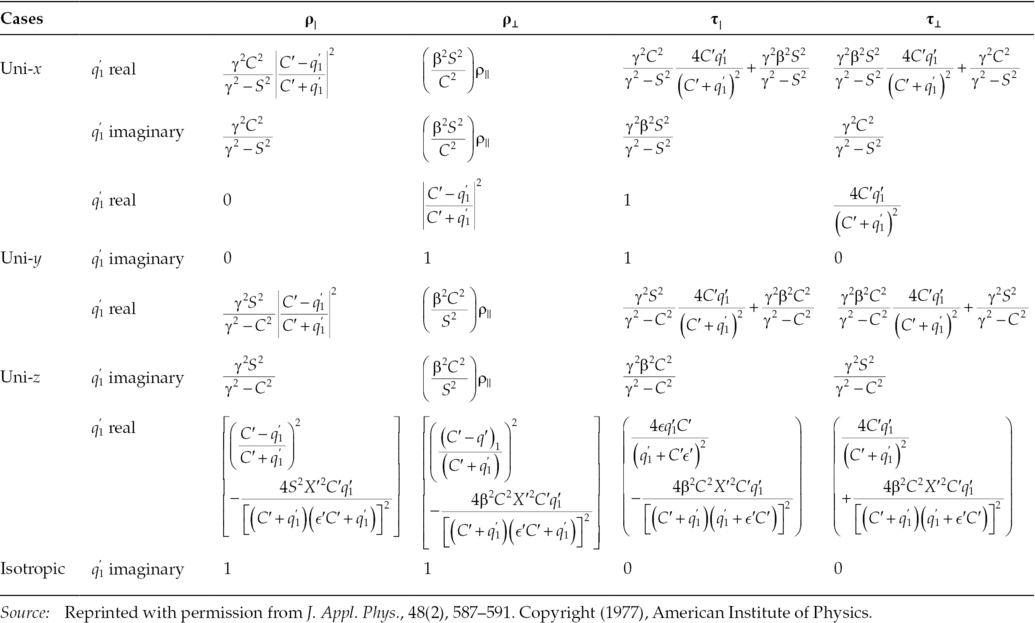
The power reflection coefficient (ρ) and the power transmission coefficient (τ) for different cases have been obtained by using Equations 14F.17 and 14F.18, for parallel as well as perpendicular polarizations, in the ranges of real and imaginary . These are given in Table 14F.1. It is found that ρ + τ = 1. The expressions for ρ⊥ and τ⊥ for an isotropic plasma given in Table 14F.1 are in agreement with the results given by Shiozawa et al. [10], when ρ⊥ and τ⊥ are deduced for a dielectric medium. The expression for ρ⊥ given in Table 14F.1 for uni-y agrees with the result given by Kong and Cheng [12]. (But the numerical results presented by them in Figure 14F.4 of their paper, for θ = 20° and 30°, show that the reflected power first increases and then decreases with β, whereas the reflected power is actually a maximum when the medium is stationary and decreases with the increase in the medium velocity.)
TABLE 14F.1
Power Reflection Coefficient (ρ) and Power Transmission Coefficient (τ) for Parallel and Perpendicular Polarization, for Various Cases
14F.4Mechanism of Power Transmission into the Plasma
Shiozawa et al. [10] decomposed the reflected and transmitted power into a contribution due to a E-wave component and an H-wave component for the case of an isotropic dielectric when the incident wave is perpendicularly polarized and showed that the sum of the H-wave component of the reflected power and the transmitted power is zero and also that the sum of the E-wave component of the reflected power and transmitted power is 1.
It is found by our analysis that for an isotropic plasma also, the same conclusions hold good when is real. But when is imaginary, the H-wave component and the E-wave component of the transmitted power are equal in magnitude and opposite in sign and hence the net power transmitted is zero and H- and E-wave components of the reflected power add to 1.
For the uni-y case, for an incident E wave (perpendicular polarization), only E waves are excited in the plasma corresponding to the mode. Thus, whenever is imaginary, the transmitted power is zero. For an incident H wave (parallel polarization), only H waves are excited in the plasma corresponding to the mode and since q′2 = C′ (q2 = C) there is a perfect match at the interface and all the incident power gets transmitted through the plasma.
For uni-x and uni-z cases, both the modes are excited in the plasma. Even if becomes imaginary (for certain ranges of wave frequency and medium velocity) and the corresponding wave is evanescent, a certain amount of power is transmitted by the second wave, being always real. The mechanism of this power transmission is examined below.
When is real, it can be shown from Equation 14F.18 for the transmitted power that is exactly equal to . Therefore, the net power contribution by these components is zero at any level in the plasma. Hence, the power contribution is from the components and and thus both the modes corresponding to and q2′ = C′ carry power.
When is imaginary, it can be shown from Equation 14F.18 that is exactly equal to . Therefore, the net power contribution by these components is zero at any level in the plasma in this case also. The power contribution by and is zero. Therefore, the power transmitted in the plasma when is imaginary is only due to the components and . This power is being carried by the mode in the plasma corresponding to the characteristic root .
14F.5Numerical Results and Discussion
The variation of ρ with the normalized wave frequency Ω = ω/ωp for the cases of uni-y, uni-x, and uni-z plasmas has been presented for different β and C = 0.5 in Figure 14F.1, Figure 14F.2 and Figure 14F.3, respectively. The variation of with Ω for β = 0 and 0. 75 and C = 0.5 has been shown as insets for the above cases. The sign of β does not affect the final results as is evident from the physical picture and also from the relevant equations where even powers of β only appear. In the case of a uni-y plasma and incident E wave (Figure 14F.1), is imaginary for 0 < Ω < 1/γ C and real for 1/γ C ≤ Ω < ∞. For a given Ω in the range Ω ≥ 1/C, is real for 0 ≤ β ≤ 1 and ρ⊥ decreases with increase in β. Further, for Ω < 1/C, is imaginary for 0 ≤ β ≤ β1 [= (1 − C2Ω2)1/2] and real for β1 ≤ β1 ≤ 1. In this range of Ω, ρ⊥ is unity for β ≤ β1 and decreases for β > β1.
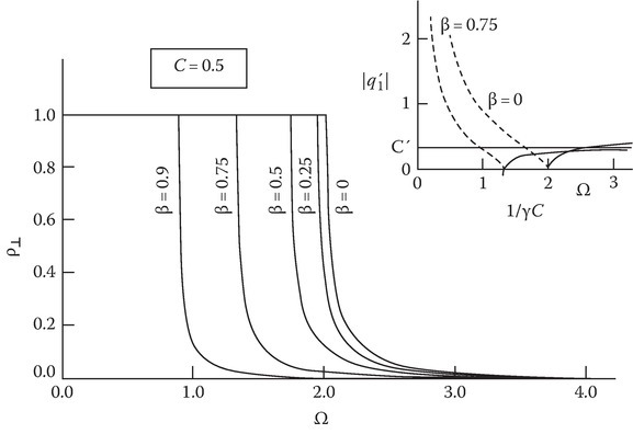
FIGURE 14F.1
Power reflection coefficient for perpendicularly polarized waves incident on a moving uni-y plasma with β as parameter. The variation of the characteristic root is shown in the inset (broken line, imaginary; solid line, real). (Reprinted with permission from J. Appl. Phys., 48(2), 587–591. Copyright 1977, American Institute of Physics.)
In the case of a uni-x plasma and incident H-wave (Figure 14F.2), is imaginary for 0 ≤ Ω ≤ Ω1 [=(1 − S1′2)1/2/C] and real for Ω < Ω ≤ ∞. In this case, three ranges of Ω are of interest. For a given Ω in the range Ω ≥ 1/C, is real for all β and ρ∥ increases with increase in β. For Ω ≤ 1, is imaginary for all β and ρ∥ decreases with increase in β. For 1 < Ω < 1/C, q1 is real for 0 ≤ β ≤ β1 [= C(Ω2 − 1)1/2/S] and imaginary for β1 ≤ β ≤ 1. In this range of Ω, ρ∥ increases with β ≤ β1 and decreases with β ≤ β1. However, ρ∥ is constant (Figure 14F.2) with Ω in the range of imaginary.
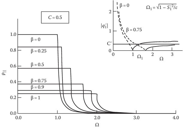
FIGURE 14F.2
Power reflection coefficient for parallel-polarized waves incident on a moving uni-x plasma with β as parameter. The variation of the characteristic root is shown in the inset (broken line, imaginary; solid line, real). (Reprinted with permission from J. Appl. Phys., 48(2), 587–591. Copyright 1977, American Institute of Physics.)
In Figure 14F.3, the case of a uni-z plasma has been presented. In this case, is imaginary for 1/γ < Ω ≤ 1/C and real in the ranges 0 < Ω < 1γ and l/C < Ω < ∞. Here also, three ranges of Ω are of interest. For a given Ω in the range Ω ≤ 1, is real for 0 < β ≤ β1 [= (1 − Ω)1/2] and imaginary for β1 < β ≤ 1. is infinity at β = β1 and zero at β = 1. In this range of Ω, ρ∥ increases first with increase in β < β1 and then decreases for β > β1. In the range 1 < Ω < 1/C, is imaginary for all β and ρ∥ decreases with β. For Ω > 1/C, is real for all β and there is an increase in ρ∥ with increase in β, but the effect is negligible and hence only one curve is shown in this range. In this case also, it is interesting to note that for imaginary, ρ∥ is constant with Ω (Figure 14F.3).

FIGURE 14F.3
Power reflection coefficient for parallel-polarized waves incident on a moving uni-z plasma with β as parameter. The variation of the characteristic root is shown in the inset (broken line, imaginary; solid line, real). (Reprinted with permission from J. Appl. Phys., 48(2), 587–591. Copyright 1977, American Institute of Physics.)
The numerical results for the isotropic plasma have not been presented here. In this case, one would see that is imaginary in the range 0 < Ω ≤ 1/C and real in the range 1/C < Ω ≤ ∞ for all β. ρ∥ is unity in the range of imaginary for all β. In the range of real, ρ∥ increases as β increases, but the effect of β is small.
Expressions are also derived for the plasma slab case and computations made showed oscillations in the range of real whose nature can be qualitatively explained as before [1,18].
Acknowledgment
The authors thank the reviewer for his valuable comments.
References
- 1.Kalluri, D. and Prasad, R. C., Appl. Sci. Res., 27, 415, 1973.
- 2.Yeh, C., J. Appl. Phys., 37, 3079, 1966.
- 3.Yeh, C., J. Appl. Phys., 38, 2871, 1967.
- 4.Lee, S. W. and Lo, Y. T., J. Appl. Phys., 38, 870, 1967.
- 5.Chawla, B. R. and Unz, H., IEEE Trans. Antenna Propag., AP-17, 771, 1969.
- 6.Kalluri, D. and Shrivastava, R. K., IEEE Trans. Antenna Propag., AP-21, 63, 1973.
- 7.Kalluri, D. and Shrivastava, R. K., J. Appl. Phys., 44, 2440, 1973.
- 8.Kalluri, D. and Shrivastava, R. K., J. Appl. Phys., 44, 4518, 1973.
- 9.Kalluri, D. and Shrivastava, R. K., IEEE Trans. Plasma Sci., PS-2, 206, 1974.
- 10.Shiozawa, T., Hazma, K., and Kumgai, N., J. Appl. Phys., 38, 4459, 1967.
- 11.Pyati, V. P., J. Appl. Phys., 38, 652, 1967.
- 12.Kong, J. A. and Cheng, D. K., J. Appl. Phys., 39, 2282, 1968.
- 13.Cheng, D. K. and Kong, J. A., Proc. IEEE, 56, 248, 1968.
- 14.Budden, K. G., Radio Waves in the Ionosphere, Cambridge University Press, Cambridge, U.K., 1961.
- 15.Derusso, P. M., Roy, R. J., and Close, C. M., State Variables for Engineers, Wiley, New York, p. 232, 1965.
- 16.Chawla, B. R., Kalluri, D., and Unz, H., Radio Sci., 2, 869, 1967.
- 17.Sommerfeld, A., Electrodynamics, Academic Press, New York, p. 287, 1964.
- 18.Kalluri, D. and Prasad, R. C., Int. J. Electron., 35, 801, 1973.