
]>
7
Miscellaneous Topics on Waves*
Most of the problems we have dealt with till now are monochromatic waves unbounded in space. Practical signals involve pulse waves or beam waves. The simple solutions obtained for monochromatic waves can be used to construct solutions for more difficult problems. In this connection, we first explore the concept of group velocity.
7.1Group Velocity vg
Group velocity is the velocity with which a group of waves travel. Let us consider that at z = 0, we have two sinusoidal oscillations:
The two oscillations differ in frequency by 2∆ω.
Equation 7.1 may be also written as
A sketch of Equation 7.2 is shown in Figure 7.1.
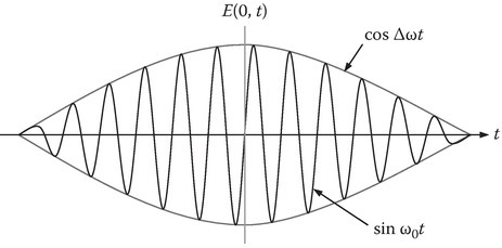
FIGURE 7.1
Two oscillations with a small beat frequency.
It shows a carrier of frequency ω0 being modulated by a signal of frequency ∆ω. The oscillation propagates as a wave that can be written as
From Equation 7.4, it is clear that while the carrier propagates with the phase velocity ω0/β0, the group travels with the group velocity:
The importance of the ω–β diagram now becomes clear. If we plot ω versus β, then the phase velocity is given by the ratio of the vertical coordinate to the horizontal coordinate, whereas the slope of the tangent gives the group velocity. If the ω–β diagram is not a straight line, then the velocity with which the members of the group travel will be different and hence the signal gets distorted. Group velocity, in many cases, is also equal to the velocity of energy transport or simply energy velocity vE defined by
where S is the power density and w the total energy density. The energy velocity represents the velocity with which the wave energy is transported.
From Equations 7.5 and 7.6, it can be shown that
Several examples of calculation of group velocity are given as problems.
7.2Green’s Function
Green’s function is the response of a system to an impulse input. In circuits, it is usually denoted by h(t), whereas in field theory it is denoted by G. The following one-dimensional problem will be solved to illustrate the essential aspects of constructing a Green’s function. G is the solution of the following differential equation:
subject to the boundary conditions
We expect G to depend on x as well as x′, that is, G = G(x, x′). Let us first solve the problem mathematically and then we will interpret the solution. Let
Since
To determine the four unknowns A1, B1, A2, and B2, we need four equations. Two are derived from the boundary conditions
We obtain two more equations from “source conditions,” at x = x′:
Equation 7.19 comes from the physics of the problem and Equation 7.20 follows from the differential equation (7.9): integrating Equation 7.9 with respect to x over the interval 0 < x < L gives
The last part of Equation 7.21 follows from the definition of the impulse function. The LHS of Equation 7.21 may be written as
Note that d2G/dx2 = 0, except for a small interval 2ε around x = x′. From Equations 7.10, 7.11, 7.19, and 7.20, we can determine A1, B1, A2, and B2. Thus, we get
Figure 7.2 shows the plot of G, dG/dx, and d2G/dx2 versus x, for the case of x′ = 2L/3.

FIGURE 7.2
Sketches of Green’s function and its derivatives: (a) G, (b) dG/dx, and (c) d2G/dx2.
Equation 7.9 is the normalized form of the differential equation of a string under tension clamped at the ends. G is the downward displacement of the string when a point load is applied at x = 2L/3. The physical picture is shown in Figure 7.3. The advantage of developing Green’s function for a problem is that the response to an arbitrary excitation may be written as a superposition integral. If the input is −f(x), for the problem, that is,
then
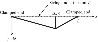
FIGURE 7.3
Clamped string under tension.
We note that Green’s function has the following properties:
It is symmetric, that is, G(x, x′) = G(x′, x).
It is continuous.
The Derivative of G has a Unit Discontinuity at x = x′. Note that the first derivative of G is one order less than the highest-order derivative in the differential equation for G.
The general procedure for constructing Green’s function may be stated as follows:
Determining the solution of the differential equation with the RHS equal to zero. The solution will involve undetermined constants.
Determining the constants using the boundary conditions and the source conditions.
Using the above, it can be shown that Green’s function G of the one-dimensional Helmholtz equation
subject to the boundary conditions,
is given by
Appendix 7A deals with the advanced aspects of the Green’s function.
7.3Network Formulation
Classical network theory deals with the interconnection of simple individual components. In the context of high-frequency electrical engineering, the individual components are wave types including transmission lines, waveguides, and cavity resonators. After briefly reviewing the network parameter description of two-port networks, the S-parameter description will be explained. Figure 7.4 shows a two-port network. The input and output variables V1, V2, I1, and I2 are related by a 2 × 2 matrix whose elements are the parameters of the network. For example,
describes open-circuit impedance parameters, called Z parameters.
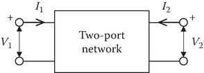
FIGURE 7.4
Two-port network.
Since Z11 = V1/I1|I2 = 0, it is the input impedance when the output is open-circuited. In the elementary circuit theory, one might have learnt about the description of a network through other parameters: short-circuit Y parameters, hybrid H parameters, and inverse hybrid G parameters. Two more sets, ABCD parameters and scattering S parameters, are particularly useful in high-frequency work. Any one set of parameters can be transformed into another set. Books on circuit theory give tables of conversion formulas. In this section, we will concentrate on ABCD parameters and S parameters.
7.3.1ABCD Parameters
The matrix definition of ABCD parameters is given by
If two networks are cascaded as shown in Figure 7.5a, then the equivalent ABCD network is as shown in Figure 7.5b, where
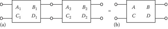
FIGURE 7.5
Networks in cascade. (a) Two networks in cascade and (b) equivalent network.
The advantage of using ABCD parameters is evident from Equation 7.33. The overall ABCD parameters of a number of two ports connected in cascade is the product of the matrices describing the individual two-port network. As a simple example of finding ABCD parameters of a two-port network, consider a series impedance Z as shown in Figure 7.6.

FIGURE 7.6
ABCD parameters of series element. (a) Series element and (b) ABCD parameters.
Since V1 = V2 + ZI1 and I1 = −I2,
Let us consider next the lossless transmission line (Figure 7.7).
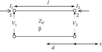
FIGURE 7.7
Lossless transmission line.
Taking the reference to be at z = 0:
Also
From Equations 7.35 and 7.36, we obtain
For a line with losses,
where γ = α + jβ is the propagation constant.
Let us next consider N transmission lines in tandem, fed by the input transmission line i and feeding the output transmission line t as shown in Figure 7.8. Then
where
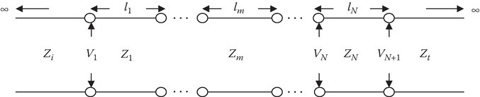
FIGURE 7.8
N transmission lines in tandem.
If V+0 is the incident voltage, Γ is the reflection coefficient, and T is the transmission coefficient, then
Arranging in a matrix form,
Solving for Γ and T yields
7.3.2S Parameters
At low frequencies only, say less than 0.5 GHz, voltage and current can be measured and ABCD parameters can be calculated. Also if the system under investigation contains active devices such as diodes or transistors, placing an open- or short-circuit calibration piece on one port, needed to measure the ABCD parameters of the device, may result in instability. The high-frequency method involves measuring incident and reflected wave quantities rather than total voltage and current. The corresponding parameters are called scattering parameters. Let us first define scattering parameters for a one-port network (Figure 7.9).
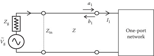
FIGURE 7.9
One-port network.
Let the incident voltage be VI1 and reflected voltage VR1. Define the normalized voltages of the incident and scattered waves as
and
The incident power is |a1|2 and the scattered power is |b1|2. At high frequencies, power measurements can be made with relative ease. Also b1 can be set to zero by matching. In the one-port case, we define
In the case of two ports (Figure 7.10), we define
and relate the b’s with a’s with the help of the scattering matrix:

FIGURE 7.10
Two-port network.
Since
the measurement is made by terminating the output side of the two-port network with a matched load (a2 = 0). S11 is the input reflection coefficient. Since
it becomes the forward transmission coefficient for the network. It measures the attenuation for passive circuits and measures the gain for an active network, say an amplifier. When the input side of the network is matched (a1 = 0), we measure S22 and S12
Here, S22 is the output reflection coefficient and S12 is the reverse transmission coefficient. Table 7.1 shows the relationship between S and ABCD parameters.
TABLE 7.1
Transformation of S–ABCD–S Parameters

It is impractical to connect measuring equipment to the two-port device under test directly. Measurements are usually carried out by introducing sections of transmission line between the device under test and the measuring equipment. These lines introduce known phase shifts, which have to be taken into account in obtaining the S parameters of the device from the measured S′ parameters:
where
In the above, γ is the propagation constant of the transmission line.
7.4Stop Bands of a Periodic Media
Equation 9.127 derived from the first principles is the dispersion relation between ω and β of a periodic medium. The results are illustrated in Figures 9.12 and 9.13. Another way of obtaining the dispersion relation, using ABCD parameters, is discussed here. As an illustration, we use two transmission lines in cascade as the two layers in a unit cell shown in Figure 7.11.
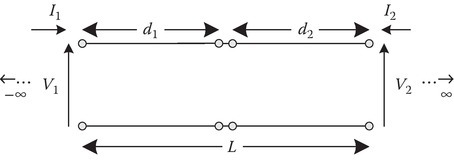
FIGURE 7.11
Unit cell of a periodic medium of infinite extent.
Let the ABCD parameters of the first transmission line be denoted by
and the second transmission line by
The overall ABCD parameters are given by Equation 7.33 relating the input voltage and current with the output voltage and current as given by Equation 7.32. However, since the medium is periodic, from Equations 9.104 and 9.105, we get
or
where
is the eigenvalue as will be shown shortly. From Equation 7.32,
From Equations 7.63 and 7.65,
The eigenvalue λ = ejβL is now determined by the eigenvalue equation
The solution for λ is given by
For a reciprocal network, AD – BC = 1. Hence,
or
A typical sketch of the ω–β diagram is shown in Figure 7.12.

FIGURE 7.12
First stop band.
Since |cos βL| ≤ 1, the edges of pass and stop bands may be located by solving
The stop and pass bands may be located by solving Equation 7.74 for ω. The first stop band shown in the figure is marked as ∆ω and is obtained by solving Equation 7.74 for βL = π. The first nonzero value shown in Figure 7.12 can arise due to the natural cutoff frequency of the unbounded medium as was the case shown in Figure 9.12.
7.5Radiation
In Section 1.3.1, we considered radiation in free space, when the source is a Hertzian dipole excited by an impulse current source. In this section, we will discuss radiation due to a time-harmonic current source. The starting point is the evaluation of Equation 1.50:
assuming that the current distribution of the source is known.
We can make some approximations based on distances [1]. If the source dimensions are of the order of d and d ≪ λ, then the field region can be classified as
The near-field (static) zone: d ≪ r ≪ λ,
The intermediate (induction) zone: d ≪ r ~ λ,
The far (radiation) zone: d ≪ λ ≪ r.
In the far zone, the term |r − r′| in the exponential of Equation 1.50 is replaced by
and the term |r − r′| in the denominator is replaced by r. This approximation can be stated as
The term outside the integral shows the spherical nature of the vector potential, and the integral term shows angular dependence.
Expanding the exponent in Equation 7.76,
If the source dimensions are of the order of d, and from our assumption that kd ≪ 1, then the dominant term is the first nonvanishing term in Equation 7.77.
If that term is n = 0 term, then
For the filamentary current, J dv′ can be replaced by I dl′:
If the filament is along the z-axis, then
For a volume source, the integrand in Equation 7.78 can be manipulated:
In order to obtain the last term in Equation 7.81, we use the continuity equation
The middle term in Equation 7.81 is obtained through integration by parts, or by evaluating one of the components:
The first term on the RHS of Equation 7.83 is zero since the current density is tangent to the surface s′. Thus, we have
From Equations 7.78 and 7.81,
where ˜pe is given by
which is called the electric dipole moment.
7.5.1Hertzian Dipole
A Hertzian dipole is a very short filament of length d, and if one considers the current to be constant, then Equation 7.79 becomes
If ˜I is considered a constant, then the continuity equation requires point charges Q and −Q at the ends of the filament. The dipole moment ˜pe of this pair of charges, when the filament is along the z-axis, is given by
Equation 7.86 gives the same result when evaluated for this very small length filament along the z-axis.
Evaluating ˜B and ˜H from the vector potential ˜A, in the far zone, we obtain
where up = c = 3 × 10⁸ m/s and η = ηo = 120π Ω for a free-space medium. The equivalence of ˜I and ˜Q are clearly seen as
In Problem P1.5, we studied the Hertzian dipole (point dipole) making the approximations of a Hertzian dipole right at the beginning of the analysis.
The result for the case of a Hertzian dipole at the origin along the z-axis, that is, ˜pe=˜I0d/jω, is given as
Since ˆr׈z=(ˆρρ+ˆzz)/r׈z=−ρˆϕ/r=−ˆϕsinθ,
The time-averaged power density is
The power coming out of a sphere of radius r is
When equated to 1/2˜I20Rrad (radiation resistance) gives
The AC resistance of the wire of radius a and conductivity σc is given by
where δ is the skin depth. For example [2], if f = 75 MHz, σc(copper) = 5.8 × 10⁷, a = 0.4 mm, and d = 4 cm, then RAC = 0.036 Ω and Rrad = 0.08 Ω. Obviously the radiation efficiency is low, in the sense that the power loss as heat is about 50% of the power radiated.
7.5.2Half-Wave Dipole
We can show that there will be a dramatic improvement in efficiency by increasing the length of the wire. To illustrate this aspect, consider a center-fed wire antenna of length λ/2. The current ˜I(z) given by
is assumed to be a standing wave, and such an assumption supported by experiments simplifies the problem. A rigorous approach requires formulation as a boundary value problem [1] (Figure 7.13).
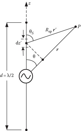
FIGURE 7.13
Half-wave center-fed dipole antenna.
A simple approach is to consider a differential length dz′ of this wire as a Hertzian point dipole. The radiated electric field in the far zone due to this differential source can be written, from Equations 7.93 and 7.94, as
In the far zone, we can make the following approximations
in the exponent.
A further approximation for Rsp in the denominator can be made:
giving
The approximations made above are equivalent to those made in Equation 7.76. Also note that in Equation 7.93, the expression for was given first and is expressed in terms of . In Equation 7.100, is given first and is then expressed in terms of [2].
The time-averaged power density in the far zone is given by
where F(θ, ϕ) is called normalized radiation intensity. Qualitatively, the pattern (Figure 7.14a) has the same features as that of the Hertzian dipole.

FIGURE 7.14
Radiation pattern F(θ) for (a) a standing wave source d = λ/2 and (b) a traveling wave source.
However, the radiated power evaluated by Equation 7.96, using Equation 7.108a, is given by
which in turn gives
In this case, Rloss of the example given for Hertzian dipole (except for changing d = λ/2) gives [2]
The efficiency of this antenna is quite good.
It can be noted that a monopole antenna with d = λ/4 over a ground plane has the same radiated fields as that of the half-wave dipole, for z > 0. The radiated power will be half of the half-wave dipole and the radiation resistance Rrad ≈ 36.5 Ω.
7.5.3Dipoles of Arbitrary Length
For an arbitrary length d relative to λ, for a center-fed antenna, the current distribution can be assumed as
And using the same technique as for the half-wave dipole, one can obtain
A plot of the radiation pattern for d = λ/2, d = λ, and d = 3λ/2 can be found in [2].
7.5.4Shaping the Radiation Pattern
Ulaby [2] gives an elementary discussion of aperture antennas, antenna arrays, and other topics of practical interest in shaping the radiation pattern.
7.5.5Antenna Problem as a Boundary Value Problem
A rigorous formulation of the antenna problem is a boundary value problem. The assumption that the current distribution is known simplifies the mathematics and allows us to compute the radiated fields. At a more basic level, what is known is the field distribution across a gap in the antenna; say, one can know the electric field in the gap. The additional boundary conditions are that the current vanishes at the end of the wires. Such a formulation is used in computational electromagnetics.
7.5.6Traveling Wave Antenna and Cerenkov Radiation
The thin-wire antenna problem discussed earlier is based on an assumed standing wave current distribution. It will be interesting to study the effect of a traveling wave current distribution.
Let be given by
The radiation vector N defined as [3] the integral,
For this case, it becomes
And the vector potential in the far zone, from Equation 7.76, is given by
Evaluating , , and Sav as before, the normalized radiation intensity for the traveling wave current excitation can be shown [3] to be
The normalized radiation intensity F(θ, ϕ) for the traveling wave source given by Equation 7.117b differs from the radiation intensity for the standing wave source given by Equation 7.112 in one important aspect. The former is asymmetrical with respect to the equatorial plane θ = π/2, whereas the latter is symmetrical. The traveling wave source creates a major lobe in the radiation pattern in the forward direction. Figure 7.14 shows the sketch of the radiation pattern for two cases.
The maximum radiation is in the neighborhood of θ = 0 and the minimum radiation is in the neighborhood of θ = π.
For the traveling wave case, the maximum radiation appears as a cone in the forward direction of the wave traveling, and the half-angle of the cone decreases as p increases or as d/λ increases.
Papas [3] points out the similarity of the conical beam radiation to that of Cerenkov radiation from fast electrons.
7.5.7Small Circular Loop Antenna
We will assume that the circumference of the loop is small compared to the wavelength. At a field point far away from the loop, the magnetic field due to steady current is similar to the electric field due to a static electric dipole.
See Section 8.9. Hence this antenna is called the magnetic dipole antenna. In applying Equation 7.114 to this case, we replace by [4]. This replacement is easily explained if we consider the coordinates of the field point as P(r, θ, 0) without loss of generality in the light of ϕ symmetry of the source.
The ϕ component of is the same as the y component of at this point. The y component of can be computed from knowing the y component of .
Thus, . Since y′ = a sin ϕ′, dy′ = a cos ϕ′ dϕ′. Moreover, in (7.114) and (7.76) is given by a cos ψ, where ψ is the angle shown in Figure 7.15 and is given by

FIGURE 7.15
Magnetic dipole antenna.
When the source is in the x–y-plane, θ′ = π/2.
For the computation of Ay, ϕ = 0 and we obtain for the case under consideration
Thus, we obtain
Assuming that ka is small, we can approximate (7.120) as
where is the magnetic dipole moment.
Computing the fields in the far zone, the time-averaged power density Sav, the total power radiated P, and equating to (1/2)I2Rrad, one can obtain [4,5]
7.5.8Other Practical Radiating Systems
Ramo et al. [4] have listed the steps involved in systemization of calculations for obtaining the radiated power, originally given by Schelkunoff [6], and applied them to many radiating systems.
7.6Scattering
Let us assume that a time-harmonic electromagnetic wave is propagating in an unbounded medium whose electric and magnetic fields are and , respectively. Let the fields be and , when a structure is present in the medium. The interaction of the incident wave (superscript i) with the structure could produce charges and currents in the structure and on the surface of the structure. These sources in turn produce scattering fields and . The total fields, in the presence of the structure, are given by
We can interpret that the scattering fields are those produced by the induced sources in the structure due to the interaction of the incident fields with the structure. The relationship between the incident fields and the induced sources in the structure can be found by using, say, the boundary conditions; as a second step, we can compute the scattered fields. Balanis [7] has several examples of such calculations. In this section, we will only do one example of such calculations, that is, the case of the two-dimensional plane wave TM (Transverse Magnetic) scattering by a circular conducting long cylinder [7].
First, we will list the relation between plane waves and cylindrical wave functions.
7.6.1Cylindrical Wave Transformations [7]
7.6.2Calculation of Current Induced on the Cylinder [7]
Let the electric field of the incident wave be
From Equation 7.124a, we have
where
The scattered field can be written as
In writing Equation 7.130, we note that the scattered field has to be an outgoing wave as βρ → ∞, and hence we choose as discussed in Section 2.15.
The PEC boundary condition at ρ = a gives
The scattered electric field is given by
The z component of the electric field at any ρ ≥ a is given by
From Maxwell’s equation,
One can obtain (note Eρ = Eϕ = 0). The component will be zero. The other tangential component can be found. The surface current K on the surface of the cylinder is given by
which comes out to be [7]
For (a ≪ λ) very thin wires, the first term is dominant:
We can approximate further by using the asymptotic value of for small βa [7]:
7.6.3Scattering Width
Scattering by the target is quantified by a parameter called echo area, radar cross section (RCS) σ. The RCS is formally defined as the area intercepting the amount of power that, when scattered isotropically, produces at the receiver a density scattered by the actual target [7]. For a three-dimensional target,
For a two-dimensional target, the parameter of interest is called scattering width, σ2D:
Since ρ → ∞, we can make far-zone approximations and replace
Evaluating Equation 7.141b [7],
where
Note the ϕ dependence of the scattering width. ϕ is the azimuthal angle of the observation point with reference to the direction of the propagation vector of the incident plane wave. Such a directional-dependent scattering width is called bistatic width.
For ϕ = 180°, it is called monostatic width or backscatter width:
For the low-frequency limit, βa is small, the n = 0 term is dominant, and
For higher frequencies, the convergence of the series in Equation 7.143 is slow. For βa = 3, six terms give satisfactory results. For βa = 100, over 100 terms are needed [8].
The moment method is successfully used to study the scattering problems of PEC and dielectric objects [9].
7.7Diffraction
Figure 7.16 shows a PEC plate with a circular hole of radius a. If a plane electromagnetic (EM) wave normally incident on it from the left is considered as a photon particle, then the photons in the circular area of radius a will go through the hole and the rest of them will be totally reflected. A circular beam of radius a will emerge into the right-half of the space. The wave front remains to be a plane as shown in Figure 7.16a. This is “the geometrical optics” approximation of the ray theory. The wave nature of the photon, however, will cause “diffraction” and cause the divergence of the beam that emerges from the hole. A diffracted ray follows a path which cannot be interpreted through reflection or refraction. Figure 7.16b shows a spherical wave front. The beam divergence can be quantified by calculating the angle θ0 [4,10] shown in Figure 7.16b. The theory of diffraction is explained through “physical optics,” making use of Maxwell equations. Various approximations are possible based on the size of (a/λ), where λ is the wavelength.
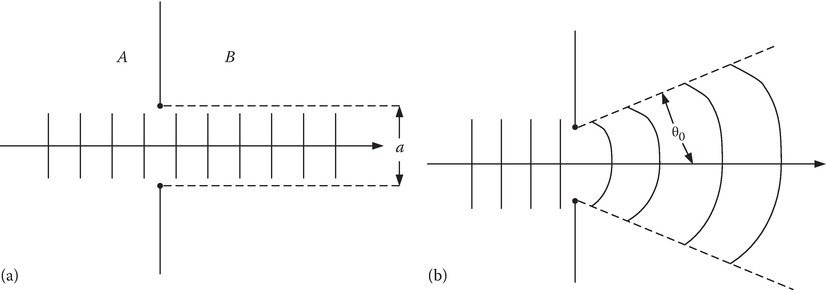
FIGURE 7.16
Propagation of the beam through a circular hole of radius a. (a) Geometrical optics. (b) Physical optics: the beam diverges.
A rigorous theory of diffraction is mathematically intense. In this section, we give the theory for the calculation of θ0 approximately. In the process, we introduce the concept of magnetic current, Jm, electric vector potential F, and the magnetic radiation vector L.
7.7.1Magnetic Current and Electric Vector Potential
Since magnetic monopoles do not exist in nature, the concept of magnetic charge density (Wb/m3) and the magnetic current density (V/m2) is artificial. However, their introduction into Maxwell equations brings out certain symmetry to the curl equations and helps us to formulate the duality theorem [7]. As we see in the next section, it also helps us to solve practical boundary value problems. The modified Maxwell equations are
The boundary conditions Equation 1.14, Equation 1.15, Equation 1.16 and Equation 1.17 will be modified as
where M (V/m) is the surface magnetic current density. The concepts M and K will be useful in replacing the tangential electric and magnetic fields in an aperture, as the one shown in Figure 7.16 and E and H are the fields on the A side of the opening. Placing the fictitious currents in the opening reduces the fields to zero in the region A and give rise, in region B, the fields that would have been there due to the original sources in region A.
Equation 1.50, when applied to a surface current source, gives us, for the time-harmonic case, the magnetic vector potential
In a source-free region,
And we can define an electric vector potential related to
The electric vector potential can be related to its magnetic current source
The fields and can be computed from and :
The middle term on the RHS of Equation 7.158 comes from the Lorentz condition:
The last term in Equation 7.158 comes from the contribution of the electric vector potential.
Equation 7.159 can be obtained on similar lines.
In Equations 7.153 and 7.157, we can substitute for and for . Thus, the potentials are given in terms of the corresponding tangential components of the fields.
We can define a magnetic radiation vector L, analogous to N given by Equation 7.114 by replacing the electric current density by the magnetic current density:
And the electric vector potential in the far zone is given by
7.7.2Far-Zone Fields and Radiation Intensity [4]
The electric and magnetic fields that do not decrease faster than 1/r are now obtained from Equations 7.158 and 7.159 as
Note that the factor ωμ/4π that appears in some of the electric formulas can also be written as
The time-averaged power density Sav can be calculated from which the total power radiated per unit solid angle dP/dΩ called radiation intensity can be calculated:
Note that the vector in Equation 7.164 is given by
When ψ, the angle between r′ and r, is expressed in terms of the spherical coordinates, we have
7.7.3Elemental Plane Wave Source and Radiation Intensity [4]
Let us consider a differential surface element ds on a uniform plane wave, having Ex and Hy and propagating in the z-direction. The equivalent current sheets have
From Equation 7.114, for a differential surface source, noting that ψ = 90°,
And from Equation 7.164, for a differential surface source,
From Equation 7.170,
Note that the plane wave differential surface source is equivalent to crossed electric and magnetic point dipoles.
7.7.4Diffraction by the Circular Hole
At the source point S(r′, π/2, ϕ′), the electric field of the uniform plane wave is given by
and since θ′ = π/2 from Equation 7.118, we have
We can compute dP/dΩ due to the fields in the circular area by integrating Equation 7.180 over the circular area:
It can be shown that
Thus,
From the integral
Equation 7.185 is evaluated:
For small θ, it is the second term in θ that establishes the pattern. A plot of bracketed term is shown in Figure 7.17.

FIGURE 7.17
Approximate form of radiation pattern of a circular aperture for small θ.
The main lobe has θ = θo, given by the first zero in the graph of Figure 7.17:
The above result is valid for ka ≫ 1 and the beam divergence is reduced by increasing a/λ and becomes zero in the limit.
The total power transmitted by the hole can be obtained from Equation 7.183:
Note that the upper limit for θ integration is θ = π/2 and not π. The incident power Pi is given by
And the power transmission coefficient is
In the two extreme cases of ka ≫ 1 and ka ≪ 1, it can be shown [1] that
Equation 7.192b has some inconsistent approximations, but shows that the transmission is small for small holes. We illustrate the order of the power transmission coefficient for a screen in the front door window of the microwave oven consumer product which has a metal screen with small holes.
At the operating frequency of 2.45 GHz (λ = 12 cm), a = 0.5 mm, from Equation 7.192b,
At microwave frequencies, the screen in the window is practically a conductor preventing the microwave radiation from escaping from the inside of the microwave oven. This is the principle of shielding using the Faraday’s case [11].
For visual frequencies, say λ = 0.5 × 10⁻⁶ m, ka ≈ 6 × 10³, and from Equation 7.192a, τ = 1. A person can easily see through the microwave oven window into the food chamber.
Schmitt [11] has illustrative graphs of simulated diffraction patterns of the radiation intensity for apertures of various widths with an incident radiation of 100 MHz (λ = 3 m), patterns measured 10 m from the aperture.
A complimentary screen to the circular aperture is a circular disk. Babinet’s principle of complementary screens [1] can be used to study the interactions with the complimentary screen in terms of the solution of the screen.
Diffraction radiation in the far zone is called Fraunhoffer diffraction. Fresnel diffraction is the radiation close to the aperture.
The rigorous treatment of scattering and diffraction are mathematically intensive and Jackson [1] and Balanis [7] have such a treatment embedded in these textbooks on electromagnetic theory.
References
- 1.Jackson, J.D., Classical Electrodynamics, 3rd edn., Wiley, New York, 1999.
- 2.Ulaby, F.T., Applied Electromagnetics, Prentice Hall, Englewood Cliffs, NJ, 2001.
- 3.Papas, C.H., Theory of Electromagnetic Wave Propagation, McGraw-Hill, New York, 1965.
- 4.Ramo, S., Whinnery, J.R., and Van Duzer, T., Fields and Waves in Communication Electromagnetics, Wiley, New York, 1965.
- 5.Lorrain, P., Corson, D.P., and Lorrain, F., Electromagnetic Fields and Waves, 3rd edn., W.H. Freeman, New York, 1988.
- 6.Schelkunoff, S.A., A general radiation formula, Proc. I.R.E., 27, 660–666, 1939.
- 7.Balanis, C.A., Advanced Engineering Electromagnetics, Wiley, New York, 1989.
- 8.Van Bladel, J., Electromagnetic Fields, McGraw-Hill, New York, 1964.
- 9.Harrington, R.F., Field Computation by Moment Methods, Macmillan, New York, 1968.
- 10.Schwarz, S.E., Electromagnetics for Engineers, Sanders College Publishing, Philadelphia, PA, 1990.
- 11.Schmitt, R., Electromagnetics Explained, Newnes, Amsterdam, the Netherlands, 2002.