
]>
Appendix 11C: Thin Film Reflection Properties of a Warm Magnetoplasma Slab: Coupling of Electromagnetic Wave with Electron Plasma Wave
11C.1Introduction
The study of interaction of electromagnetic waves with warm magnetoplasma continues to attract the attention of researchers in electromagnetics [1]. Earlier research in the 1960s and 1970s was motivated by its possible application (1) in opening the passband below plasma frequency for the problem of radio reentry blackout [1] and (2) RF heating of fusion plasmas [2,3]. There is a resurgence of research in this area due to new applications. The broad area of plasmonics, which utilizes the coupling of electromagnetic waves with an electron plasma wave, has applications in (1) HEMT [4,5,6] and in the general area of (2) plasma wave electronics [7,8,9,10]. The important features of the interaction can be obtained by studying the reflection and transmission properties of a warm magnetoplasma slab.
Numerical results for a general problem of oblique incidence of an electromagnetic plane wave on a warm, thin magnetoplasma slab [2,11] with different input and output media can be obtained by formulating it as a boundary value problem. Reference 1 gives a detailed study of this aspect.
To interpret and explain the results—by unraveling the effects of various parameters given in Table 11C.1 on the (a) behavior near resonances, (b) behavior due to triply refractive magnetoplasma medium, (c) excitation of evanescent and/or propagating positive-going or negative-going waves in various frequency bands, (d) tunneling of power through a thin slab in the stop bands [12,13,14,15,16], and (e) excitation of surface plasmons [13,17]—requires simpler formulations that bring out each of these consequences into focus. Characterizing reflection properties for a magnetoplasma slab can be achieved by careful choice of various parameters in Table 11C.1.
TABLE 11C.1
Parameters of Interest for a Warm Magnetoplasma Slab

Consider first the simpler case of isotropic, warm plasma slab. For normal incidence, it is obvious that electron plasma wave (which requires electric field in z-direction) will not be excited in the slab. For oblique incidence, the electromagnetic as well as electron plasma wave will be excited in the slab, and the results for this case are discussed in [13] and Appendix 10A.
For normal incidence of R wave (right circular polarization) or L wave (left circular polarization), when the static magnetic field is in the z-direction, the electron plasma wave will not be excited [18], and the results for cold or warm magnetoplasma slab are the same. For normal incidence of x- or y-polarized wave, when the static magnetic field is in the z-direction, the results of cold and warm plasma slab are the same since the linear polarization in x- or y-direction can be considered as a superposition of R and L waves. For normal incidence of y-polarized wave, when the static magnetic field is in the y-direction, the results are the same as those of isotropic plasma slab.
For normal incidence of x-polarized wave, when the static magnetic field is in the y-direction, the results are very different for the cold and warm plasmas. The incident electromagnetic wave excites in the plasma an extraordinary wave (called X wave) [12] with the results for warm and cold cases very different near upper hybrid frequency ωuh. For the warm plasma case, the resonance (refractive index infinity) for the cold case will be replaced by a finite value for the refractive index. In the neighborhood of the upper hybrid frequency, the characteristic of the waves in the magnetoplasma will change from a basically electromagnetic wave to that of an electron plasma wave [17]. In this appendix, we formulate and solve the associated electromagnetic boundary value problem to study this aspect of coupling of the waves and the effect of various parameters on the coupling. Moreover, the role of the evanescent waves on the tunneling of power through a thin slab will be explored.
11C.2Formulation of the Problem
The power reflection coefficient in this chapter is derived from detailed equations starting with Maxwell’s equations and the hydrodynamic approximation. The wave equation for a warm, compressible, anisotropic magnetoplasma was derived by Unz [19].
To describe the electromagnetic waves inside the slab, the medium is modeled as a lossless (collisionless), homogeneous, anisotropic () warm plasma of thickness d. The plasma slab of np is bounded by two half-space media n = 1. The incident wave is x-polarized, equivalent to normal incidence (θI = 0) of a parallel-polarized (TM or p) wave (see Figure 11C.1). In addition, there is a magnetostatic field normal to the plane of incidence, or .
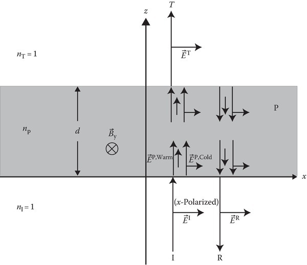
FIGURE 11C.1
Normal incidence of an x-polarized wave on a warm, anisotropic plasma slab. Shown are the reflection and transmission waves. I, incident; R, reflected; T, transmitted, P, plasma.
11C.2.1Waves Outside the Slab
For the incident, reflected, and transmitted (I, R, and T) waves outside the plasma slab, the incident wave can be described as follows:
where η0 = k0/ωμ0.
11C.2.2Waves Inside the Slab (Cold Plasma)
Using the exponential factor,
where , for i = 1, 2. Note: For normal incidence, qi = np , i. From [12], the dielectric constant for an X wave in an anisotropic plasma is
Equation 11C.3 agrees with [15] for normal incidence dispersion relation when normalizing ω and ωb by the plasma frequency ωp: Ω = ω/ωp, Ωb = ωb/ωp and by allowing X = Ω−2 with Y = ω/ωb. It also agrees with Appleton–Hartree formula for a wave at normal incidence on a collisionless cold plasma as described by Budden [20]. The dielectric constant can also be written in terms of cutoff and upper hybrid frequencies:
When (11C.4) is normalized,
The upper hybrid frequency, and its normalized file are given by
For an anisotropic plasma where the magnetostatic B0 field is normal to the plane of incidence, the X wave is propagating transversely to the B0 field. From [12], the x-component is preserved, but there is also a z-component; hence, for i = 1, 2,
where ηp , i = η0/qi. From Equations 11C.1 and 11C.7 and using tangential boundary conditions, for z = 0 and d, one can derive the power reflection coefficient:
where dp is the normalized film thickness and dp = d/λp, λp is the normalized plasma wavelength.
11C.2.3Waves Inside the Slab (Warm Plasma)
The symbols used for the parameters of warm plasma medium are given in Table 11C.2. The basic equations for a warm plasma are Maxwell’s equations:
TABLE 11C.2
Warm Plasma Parameters
Using the hydrodynamic approximation for a compressible electron gas, the conservation of momentum [19] is given as follows:
The conservation of energy is given by
The equation of state is given by
The formulation given above is based on linear theory. Unz showed that Equations 11C.9 and 11C.10 reduce to the wave equation
In the above
where Z is given in terms of the electron collision frequency ν and the transmission frequency ω:
Also e is the absolute value of the charge and m is the mass of the electron. The normalized velocity variable
where a is the acoustic velocity of the electron plasma wave and np is the plasma refractive index. The electric and magnetic field intensities inside the plasma can be described as
The phase of the fields within the plasma slab is defined as
For normal incidence, np = q and . When using (11C.14) and (11C.15) in (11C.10a), one has for normal incidence on the slab interface the dispersion relation
The first term is the dispersion relation for an O wave for an electric field within the plasma in the y-direction. The second term in the {} is the dispersion relation for the X wave. Although solvable, the solution in the second term cannot be decoupled between cold and warm plasmas; however, for a solution of q1 , 2|δ → 0, Equation 11C.3 would result and q3 , 4|δ → 0 has no physical significance.
We use boundary conditions where the tangential components of and are continuous at z = 0 and d to generate four equations. For time-harmonic waves, tangential boundary conditions are used as they are derived by Maxwell’s curl equations. Normal boundary conditions (from divergence equations) can be derived from the curl equations. Hence, normal boundary conditions are not independent but are assured to be satisfied when the tangential boundary conditions are satisfied [21]. Using a scalar electron pressure, hydrodynamic approach, it is assumed that the electron velocity normal to the plasma/dielectric boundary is zero [11,21,22], which results in two more boundary equations. However, we do not assume electron pressure to be zero at the boundaries. Writing the system of equations from the boundary conditions, solving and one has the power reflection coefficient for a warm magnetoplasma,
where
In (11C.17b) and (11C.17d), ϕ1 = 2πdpΩq1 and ϕ3 = 2πdpΩq3. Note how Equation 11C.17a compares with Equation 11C.8 and yet considerably more complex as a result of the warm plasma medium even when it is modeled by hydrodynamic approximation.
11C.3Characteristic Roots and the Power Reflection Coefficient
The hydrodynamic approximation takes into account that electron plasma wave has a velocity high enough where the plasma is considered compressible. When the acoustic mode velocity approaches zero, the plasma becomes cold and incompressible. The longitudinal characteristic roots are dependent on the parameter δ = a/c, where a is the acoustic velocity of the electron plasma wave. In certain metals, the Fermi velocity [17] plays the role of the acoustic velocity. When a is comparable to c, that is, δ ≈ 0.1 – 0.01, the plasma is spatially dispersive and is considered to be warm. A small percentage change in the velocity of the longitudinal component gives rise to a dynamic response of the power reflection coefficient. In addition, the oscillations (or resonances) within the warm plasma reflection coefficient tend to ride atop the cold plasma component.
A method to understand the reflection properties is to examine the dispersion relation, which when solved leads to the characteristic roots of the plasma medium. Note that we consider here the lossless case, U = 1, where the characteristic roots are either real or imaginary but not complex. For the anisotropic case, X wave only, there are four roots to consider, q1 , 2 and q3 , 4, which create four distinct regions that affect ρ. In our previous paper [13], the regions of the power reflection coefficient were defined by the cutoff frequencies (zeros of q). In this paper, the regions are defined by the cutoff and upper hybrid frequencies.
Figure 11C.2 shows the results of Equations 11C.5 (cold) and 11C.17a (warm) power reflection coefficients. The bottom smaller plots separate the two for clarity. There is a considerable difference between the cold and warm plasma reflection coefficients. This is a result of an Ez component that excites longitudinal propagation (acoustic mode), which is a solution to the wave equation.
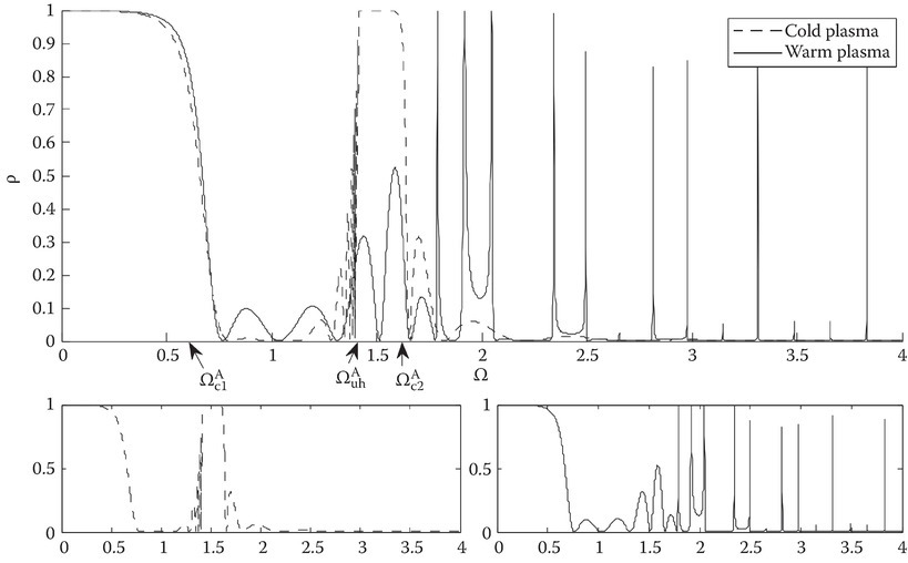
FIGURE 11C.2
Power reflection coefficient for dP = 1, δ = 0.1, θI = 0°, Ωb = 0.5, and nI = nT = 1.
Figures 11C.3 and 11C.4 show the characteristic roots for the cold and warm plasma models. From Equation 11C.3, a resonance would occur when 1 − X − Y2 = 0 for the cold plasma, that is, qi → ∞ [18] determines that the resonance was located at X = 1 − Y2. This produced Equation 11C.8, which was determined here as the upper hybrid frequency. The resonance is located in the region where the approximations to warm plasma dispersion equations fail [18]. For the warm plasma, the characteristic root qi will not go to infinity when 1 − X − Y2 = 0 and remove the resonance in the cold plasma model. To ascertain the exact value of qi at the resonance region from the second term of Equation 11C.16 yields the characteristic root at the upper hybrid frequency
where Yuh = Ωb/Ωuh and . The negative sign gives the value for and leads to an evanescent wave. Equation 11C.18 is equivalent to the “true point” that Tanenbaum [18] describes. For a warm plasma, at the upper hybrid frequency, there exists a true point that replaces a resonance as shown in Figure 11C.3, in magnetoionic plasma theory. Hence, there is a transition from a transverse electromagnetic wave to a longitudinal electroacoustic wave.
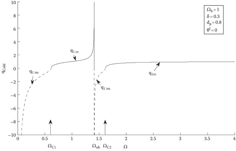
FIGURE 11C.3
Cold plasma characteristic roots for θI = 0°. The resonance is at the upper hybrid frequency Ωuh = 1.414. The cutoff frequencies are ΩC1 = 0.618 and ΩC2 = 1.618; dotted, imaginary; solid, real.

FIGURE 11C.4
Warm plasma characteristic roots; dotted, imaginary; solid, real.
To qualitatively understand the dynamics inside the plasma, one can look at how the characteristic roots change in frequency space. Fundamental changes in qi occur at the cutoff points ΩC1 , C2 and the upper hybrid frequency Ωuh (Equation 11C.5).
11C.3.1Regions of the Power Reflection Coefficient
For 0 < Ω < ΩC1: Both q1 and q3 are imaginary, noted as dashed lines in Figures 11C.3 and 11C.4. This means that both the electromagnetic and electroacoustic waves do not propagate and are evanescent. The power reflection coefficient is close to unity as all the energy is reflected back (Figure 11C.5). A unity value of ρ means ξ1 ≈ 0, and by looking at Figure 11C.4 as Ω → 0, both q1 and q3 are very large and negative and can be considered approximately equal. Both terms in ξ1 can be shown to be zero if q1 = q3. However, the reflection coefficient starts on a downward path as Ω → Ωc1. This downward path also shows the deviation between the cold and warm results. The deviation results as Ω approaches the first cutoff frequency and q1 can no longer be considered equal to q3; therefore, ξ1 ≠ 0.
For ΩC1 < Ω < ΩC2: There are two subregions to consider, as the characteristic roots cross over the upper hybrid frequency and wave coupling occurs.
For ΩC1 < Ω < Ωuh: From Figure 11C.4, q1 is real and q3 is imaginary, and the electromagnetic wave now propagates through the slab, while the electroacoustic wave remains evanescent. As a result, from Equation 11C.7a, Ep , z , i is small. The electromagnetic propagation presents itself by observing that the power reflection coefficient for both the cold and warm results starts to oscillate. The cold plasma result oscillates at increasing rates before a sharp rise at Ω = Ωuh = 1.414, then stops oscillating (Figure 11C.6). The warm plasma also oscillates albeit at a slow rate almost following the cold plasma result until the cold plasma result oscillates faster on its own.
For Ωuh < Ω < ΩC2: From Figure 11C.4, q1 is imaginary and q3 is real, and the electroacoustic mode now propagates through the slab, while the electromagnetic wave remains evanescent and Ep , z , i becomes large. This is possible as a result of the coupling of the electroacoustic wave to the electromagnetic wave at the true points; hence, Ω = Ωuh. The cold plasma power reflection coefficient remains constant reflecting the electromagnetic wave in this region, but the warm plasma part continues to oscillate by propagating the electroacoustic wave (Figure 11C.7).
For ΩC2 < Ω < ∞: Both q1 and q3 are real, shown as solid lines in Figures 11C.3 and 11C.4. Both the electromagnetic and electroacoustic waves are propagating through the slab. For the power reflection coefficient, the warm plasma resonances ride atop of the smooth, cold plasma result, which could be qualitatively described as Tonks–Dattner resonances (Figure 11C.8) [13].
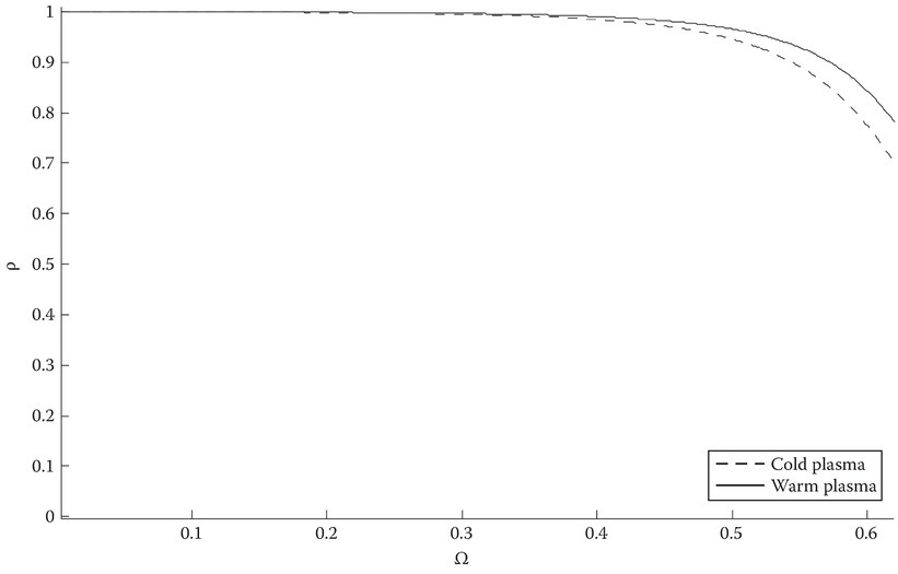
FIGURE 11C.5
The power reflection coefficient ρ for 0 < ΩC1.

FIGURE 11C.6
The power reflection coefficient ρ for ΩC1 < Ω < Ωuh.
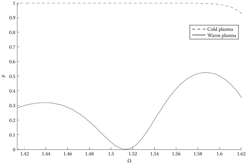
FIGURE 11C.7
The power reflection coefficient ρ for Ωuh < Ω < ΩC2.
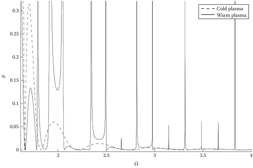
FIGURE 11C.8
The power reflection coefficient ρ for ΩC2 < Ω < ∞.
11C.3.2Other Cases of the Power Reflection Coefficient
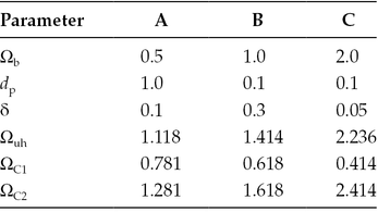
Variations of the power reflection coefficient are shown with different magnetic field strengths as well as different δ’s and film thicknesses. Three cases are chosen and described in Table 11C.3 to show how the power reflection coefficient changes with variations in the physical parameters in the table and, more importantly, how the cold and warm plasma power reflection coefficients change for the same parameters.
TABLE 11C.3
Different Cases A, B, and C of Parameters
For case A, the film thickness is same as the plasma wavelength, λp. In the low frequency range the characteristic roots for both cold and warm cases are very large in the negative direction and are negative imaginary (Figure 11C.9 and 11C.10). Both the cold and warm power reflection coefficients follow each other fairly well with ρ ≈ 1, and no energy propagates through the slab (Figure 11C.11). As Ω → ΩC1, the characteristic roots are small and ρ starts to trend downward and is approximately 0.9 at ΩC1. For Ωb = 0.5, there is a cold plasma resonance at the upper hybrid frequency Ωuh = 1.118 (Figure 11C.9). Between ΩC1 and Ωuh, the cold plasma characteristic root becomes real and transverse waves will propagate through the slab. The power reflection coefficient for both cold and warm models will continue to track each other and oscillate.
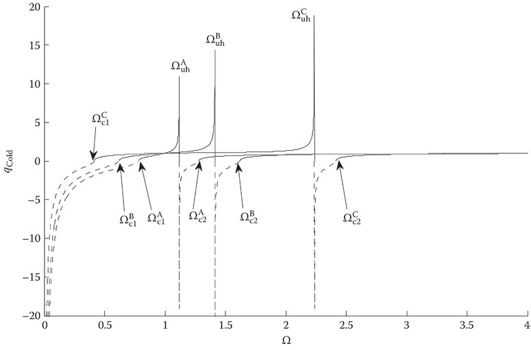
FIGURE 11C.9
Cold plasma model; characteristic roots for cases A, B, and C. The junction between the dotted and solid lines are marked with the cutoff or resonant frequencies.
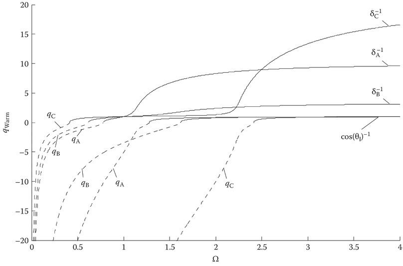
FIGURE 11C.10
Warm plasma model; characteristic roots for cases A, B, and C.
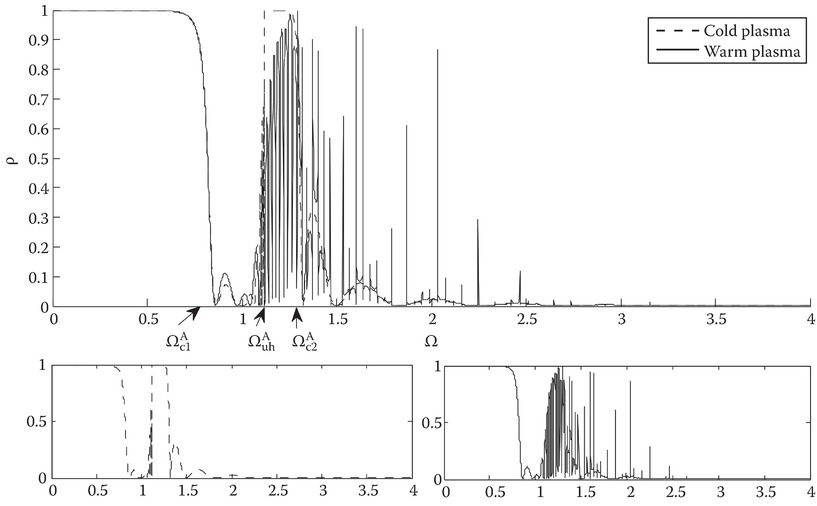
FIGURE 11C.11
Case A, Ωb = 0.5, dp = 1.0, and δ = 0.1.
However, as Ω → Ωuh, the cold plasma power reflection coefficient will oscillate at increasing rates until it reaches the upper hybrid frequency, then steps up to 1, where as the warm plasma coefficient will continue to oscillate but increases its rate slowly through the upper hybrid frequency. At Ωuh, the transition from transverse waves to longitudinal waves and vice versa takes place, and the characteristic roots resolve the resonance with true points at 2.0252 and i1.9752. The cold characteristic root now becomes imaginary and the warm is real; thus, electrostatic waves only propagate. The cold power reflection coefficient rises sharply from 0 to 1 after oscillating. The warm power reflection coefficient doesn’t necessarily track the cold plasma part but oscillates under the portion of the cold plasma that looks like a step function. At the second cutoff frequency, ΩC2, both characteristic roots are real and both transverse and longitudinal waves propagate through the slab. The cold plasma power reflection coefficient dips down to zero, then slowly oscillates, while the warm counterpart continues to oscillate, yet it tracks the cold component and its oscillations tend to ride atop of the cold plasma results similar to the Tonks–Dattner resonances [22] counterpart. When Ω → ∞, the cold characteristic root tends to 1 and the warm tends to δ−1.
For case B (Figure 11C.12), the normalized electron gyrofrequency, proportional to the strength of the static magnetic field, Ωb = 1. From Figures 11C.8 and 11C.9, we see that increasing the magnetostatic field shifts the resonance of the cold plasma characteristic root as well as the warm plasma true points to the right. The film thickness is one-tenth of the plasma wavelength and δ = 0.3. The power reflection coefficient takes on a different behavior when compared to case A. The behavior of the characteristic roots is similar in all cases, and they will not be repeated. The power reflection coefficient between 0 and ΩC1 tends downward with clear difference between the cold and warm models. When Ω → Ωuh, the ρ of the cold model tends upward with a sharp dip to 0 just before Ωuh = 1.414, then upwards again, while the warm model continues toward 0, and then hits two resonances at 2.07 and 3.31.
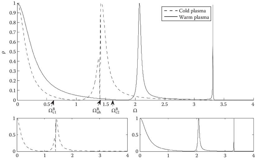
FIGURE 11C.12
Case B, Ωb = 1.0, dp = 0.1, and δ = 0.3.
For case C, the normalized B field strength is Ωb = 2, and although there are distinct differences between cold and warm power reflection coefficients (Figure 11C.13) from 0 to ΩC1, they both trend down to ρ = 0 until the warm characteristic root becomes appreciably small. “As the warm plasma characteristic root approaches 0 or Ω → Ωuh, the cold and warm plasma power reflection coefficients trend upward but start to oscillate. The cold plasma power reflection coefficient rises up to and the warm plasma counterpart continues to oscillate until Ω reaches ΩC2. Beyond the second cutoff frequency, ρ for the cold plasma monotonically decreases to 0 while the ρ for the warm plasma oscillates atop it”. These corrections are not shown on the corrected page proofs file.

FIGURE 11C.13
Case C, Ωb = 2.0, dp = 0.1, and δ = 0.05.
11C.4Conclusion
Reflection properties for a thin metal slab with an incident X wave have been presented with emphasis on the power reflection coefficient and its corresponding characteristic roots. The film was modeled as a cold and warm plasma that supports a longitudinal electromagnetic acoustic mode, which is a solution to Maxwell’s equations. For the X wave, the cold and warm plasma results differ greatly where there would be no difference for (R–L–O–) waves. The characteristic roots show that the warm plasma resolves the resonance at the upper hybrid frequency at a true point, and in frequency space, a transition occurs where a transverse wave is coupled to a longitudinal wave and vice versa. The power reflection coefficient changes behavior as a result of the wave coupling and frequency cutoff points.
References
- 1.Markos, C. T., Thin film reflection properties of warm anisotropic plasma slabs, PhD thesis, University of Massachusetts Lowell, Lowell, MA, 2012.
- 2.Kalluri, D. K., Numerical solutions of electromagnetic waves in inhomogeneous magnetoplasma slabs, PhD thesis, University of Kansas, Lawrence, KS, 1968.
- 3.Miyamoto, K., Plasma Physics for Nuclear Fusion, Revised edition, The MIT Press, Cambridge, MA, 1987.
- 4.Shur, M. S. and Lu, J. Q., Terahertz sources and detectors using two-dimensional electronic fluid in high electron-mobility transistors, IEEE Trans. Microw. Theory Tech., 48(4), 750–756, 2000.
- 5.Kushwaha, M. S. and Vasilopoulos, P., Resonant response of a FET to an AC signal: Influence of magnetic field, device length, and temperature, IEEE Trans. Electron Dev., 51(5), 803–813, 2004.
- 6.Muravjov, A. V., Veksler, D. B., Hu, X., Gaska, R., Pala, N., Saxena, H., Peale, R. E., and Shur, M. S., Resonant terahertz absorption by plasmons in grating-gate GaN HEMT structures, Proc. SPIE, 7311, 73110D-1–73110D-7, 2009.
- 7.Shur, M., AlGaN/GaN plasmonic terahertz electronic devices, 2014, J. Phys.: Conf. Ser. 486 012025. http://iopscience.iop.org/1742-6596/486/1/012025. Accessed on August 16, 2017.
- 8.Fourkal, E., Velshev, I., Ma, C.-M., and Smolyakov, A., Evanescent wave interference and the total transparency of a warm high-density plasma slab, Phys. Plasmas, 13, 092113 (2006); doi: http://dx.doi.org/10.1063/1.2354574. Accessed on August 17, 2017.
- 9.Smolyakov, A. I., Fourkal, E., Krasheninnnikov, S. I., and Sternberg, N., Resonant modes and resonant transmission in multi-layer structures, Prog. Electromagn. Res., 107, 293–314, 2010.
- 10.Yesil, A. and Aydogdu, M., The effect of the electron sound speed on wave propagation in the ionospheric plasma, Acte Geophys., 59(2), 398–406, April 2011.
- 11.Chawla, B. R., Kalluri, D., and Unz, H., Propagation of oblique electromagnetic waves through a plasma slab with normal magnetostatic field, Radio Sci., 2, 869–879, 1967.
- 12.Kalluri, D., Electromagnetic Waves, Materials, and Computation with MATLAB, CRC Press, Boca Raton, FL, 2011.
- 13.Markos, C. T. and Kalluri, D., Thin film reflection properties of a warm isotropic plasma slab between two half-space dielectric media, J. Infrared Millim. Terahertz Waves, 32(7), 914–934, 2011.
- 14.Kalluri, D. K. and Prasad, R. C., Thin-film reflection properties of isotropic and uni-axial plasma slabs, Appl. Sci. Res., 27, 415–424, 1973.
- 15.Kalluri, D. and Prasad, R. C., Thin-film reflection properties of an anisotropic plasma slab immersed in a static magnetic field normal to the plane of incidence, Int. J. Electron., 35(6), 801–816, 1973.
- 16.Prasad, R. C., Transient and frequency response of a bounded plasma, PhD thesis, Birla Institute of Technology, Ranchi, India, 1976.
- 17.Forstmann, F. and Gerhardts, R. R., Metal Optics Near the Plasma Frequency, Springer-Verlag, Berlin, Germany, pp. 9–24, 1986.
- 18.Tanenbaum, B. S., Plasma Physics, McGraw-Hill Book Company, New York, NY, pp. 122–129, 1967.
- 19.Unz, H., Oblique wave propagation in a compressible general magnetoplasma, Appl. Sci. Res., 16, 105–120, 1965.
- 20.Budden, K. G., Radio Waves in the Ionosphere: The Mathematical Theory of the Reflection of Radio Waves from Stratified Ionised Layers, Cambridge University Press, New York, NY, p. 144, 1966.
- 21.Crawford, F. W., Internal resonances of a discharge column, J. Appl. Phys., 35, 1365–1369, 1964.
- 22.Vandenplas, P. E., Electron Waves and Resonances in Bounded Plasmas, Interscience Publishers, New York, NY, p. 29, 1968.