Search in book...
Toggle Font Controls
Create new playlist

Name your new playlist

Playlist description (optional)
Sign In

Email address

Password

Forgot Password?

or

Continue with Facebook

Continue with Google
Sign Up

Full Name

Email address

Confirm Email Address

Password

or

Continue with Facebook

Continue with Google

Two-Dimensional Problems and Waveguides

3
Two-Dimensional Problems and Waveguides

In the previous chapter, we examined one-dimensional solutions. We found the solutions to be plane or cylindrical TEM (transverse electric and magnetic) waves. The TEM waves are the simplest kind of electromagnetic waves.

The next level of simple waves is either transverse magnetic (TM) or transverse electric (TE). Such waves arise when the wave is confined (bounded) in the transverse plane with, say, conducting boundaries, and is traveling in a direction normal to the transverse plane.

3.1Two-Dimensional Solutions in Cartesian Coordinates

Let us investigate the solution of Maxwell’s equations under the following constraints: (1) the wave is traveling in the z-direction, (2) it has an electric field component in the z-direction, (3) there are no sources in the region of interest, and (4) the medium in the region of interest is lossless.

The E˜z ${\tilde{E}}_{z}$ component satisfies the equation

(3.1)

\nabla 2 E ˜ z + k 2 E ˜ z = 0,

$\nabla^{2} {\tilde{E}}_{z} + k^{2} {\tilde{E}}_{z} = 0,$

where

(3.2)

k 2 = ω 2 μ ε .

$k^{2} = ω^{2} μ ε .$

Let

(3.3)

E ˜ z (x, y, z) = F (x, y) e - γ z .

${\tilde{E}}_{z} (x, y, z) = F (x, y) e^{- γ z} .$

The wave is a positive-going traveling wave when γ is imaginary, that is, γ = jβ, where β is real and positive. It is an attenuating wave when γ is purely real, that is, γ = α, where α is real and positive. Since the medium is assumed lossless, the attenuation in this case is due to the fact that the wave is evanescent. We will confirm this after we complete the solution.

Substituting Equation 3.3 into Equation 3.1, we obtain

(3.4)

\partial 2 F \partial x 2 + \partial 2 F \partial y 2 + k 2 c F = 0,

$\frac{\partial^{2} F}{\partial x^{2}} + \frac{\partial^{2} F}{\partial y^{2}} + k_{c}^{2} F = 0,$

where

(3.5)

k 2 c = k 2 + γ 2 .

$k_{c}^{2} = k^{2} + γ^{2} .$

Separation of variable method is a standard technique of solving this partial differential equation (PDE). The technique converts the PDE into ordinary differential equations (ODEs) with a constraint on the separation constants. The meaning becomes clear as we proceed. Let F be expressed as a product of two functions

(3.6)

F (x, y) = f 1 (x) f 2 (y),

$F (x, y) = f_{1} (x) f_{2} (y),$

where f₁ is entirely a function of x and f₂ is entirely a function of y. Substituting Equation 3.6 into Equation 3.4, we obtain

(3.7)

1 f 1 \partial 2 f 1 \partial x 2 + 1 f 2 \partial 2 f 2 \partial y 2 + k 2 c = 0.

$\frac{1}{f_{1}} \frac{\partial^{2} f_{1}}{\partial x^{2}} + \frac{1}{f_{2}} \frac{\partial^{2} f_{2}}{\partial y^{2}} + k_{c}^{2} = 0.$

Differentiating partially with respect to x, we obtain

(3.8)

\partial \partial x [1 f 1 \partial 2 f 1 \partial x 2] = 0,

$\frac{\partial}{\partial x} [\frac{1}{f_{1}} \frac{\partial^{2} f_{1}}{\partial x^{2}}] = 0,$

(3.9)

1 f 1 \partial 2 f 1 \partial x 2 = constant .

$\frac{1}{f_{1}} \frac{\partial^{2} f_{1}}{\partial x^{2}} = constant .$

Let this constant be denoted by −k2x $- k_{x}^{2}$ . Equation 3.9 may be written as

(3.10)

d 2 f 1 d x 2 + k 2 x f 1 = 0.

$\frac{d^{2} f_{1}}{d x^{2}} + k_{x}^{2} f_{1} = 0.$

Following the same argument, the second term in Equation 3.7 can be equated to −k2y, $- k_{y}^{2},$ leading to the ODE

(3.11)

d 2 f 2 d y 2 + k 2 y f 2 = 0.

$\frac{d^{2} f_{2}}{d y^{2}} + k_{y}^{2} f_{2} = 0.$

From Equation 3.7, we can see that the constants k2x $k_{x}^{2}$ and k2y $k_{y}^{2}$ are subject to the constraint

(3.12)

k 2 x + k 2 y = k 2 c .

$k_{x}^{2} + k_{y}^{2} = k_{c}^{2} .$

The PDE (Equation 3.4) is converted into the two ODEs given by Equations 3.9 and 3.10 subject to the constraint given by Equation 3.12. Each ODE has two independent solutions. If the constants k2x $k_{x}^{2}$ and k2y $k_{y}^{2}$ are negative, that is,

(3.13)

k 2 x = - K 2 x,

$k_{x}^{2} = - K_{x}^{2},$

(3.14)

k 2 y = - K 2 y,

$k_{y}^{2} = - K_{y}^{2},$

where K2x $K_{x}^{2}$ and K2y $K_{y}^{2}$ are positive, then the solutions are hyperbolic functions. Thus, the admissible functions are

(3.15)

f 1 (x) = ⎧ ⎩ ⎨ ⎪ ⎪ ⎪ ⎪ ⎪ ⎪ ⎪ ⎪ ⎪ ⎪ ⎪ ⎪ ⎪ ⎪ ⎪ ⎪ ⎪ ⎪ ⎪ ⎪ ⎪ ⎪ ⎪ ⎪ ⎪ ⎪ ⎪ ⎪ ⎪ ⎪ sin k x x cos k x x e + j k x x e - j k x x sinh K x x cosh K x x e + K x x e - K x x ⎫ ⎭ ⎬ ⎪ ⎪ ⎪ ⎪ ⎪ ⎪ ⎪ ⎪ ⎪ ⎪ ⎪ ⎪ ⎪ ⎪ ⎪ ⎪ ⎪ ⎪ ⎪ ⎪ ⎪ ⎪ ⎪ ⎪ ⎪ ⎪ ⎪ ⎪ ⎪ ⎪,

$f_{1} (x) = \{\begin{array}{c} sin k_{x} x \\ cos k_{x} x \\ e^{+ j k_{x} x} \\ e^{- j k_{x} x} \\ sinh K_{x} x \\ cosh K_{x} x \\ e^{+ K_{x} x} \\ e^{- K_{x} x} \end{array}\},$

(3.16)

f 2 (y) = ⎧ ⎩ ⎨ ⎪ ⎪ ⎪ ⎪ ⎪ ⎪ ⎪ ⎪ ⎪ ⎪ ⎪ ⎪ ⎪ ⎪ ⎪ ⎪ ⎪ ⎪ ⎪ ⎪ ⎪ ⎪ ⎪ ⎪ ⎪ ⎪ ⎪ ⎪ ⎪ ⎪ sin k y y cos k y y e + j k y y e - j k y y sinh K y y cosh K y y e + K y y e - K y y ⎫ ⎭ ⎬ ⎪ ⎪ ⎪ ⎪ ⎪ ⎪ ⎪ ⎪ ⎪ ⎪ ⎪ ⎪ ⎪ ⎪ ⎪ ⎪ ⎪ ⎪ ⎪ ⎪ ⎪ ⎪ ⎪ ⎪ ⎪ ⎪ ⎪ ⎪ ⎪ ⎪ .

$f_{2} (y) = \{\begin{array}{c} sin k_{y} y \\ cos k_{y} y \\ e^{+ j k_{y} y} \\ e^{- j k_{y} y} \\ sinh K_{y} y \\ cosh K_{y} y \\ e^{+ K_{y} y} \\ e^{- K_{y} y} \end{array}\} .$

The solution to a given problem may be constructed by choosing a linear combination of the admissible functions. The choice is influenced by the boundary conditions. An illustration is given in the following section.

3.2TM_mn Modes in a Rectangular Waveguide

Figure 3.1 shows the cross section of a rectangular waveguide with conducting boundaries (PEC) at x = 0 or a and y = 0 or b. TM modes have ${\tilde{E}}_{z} \neq 0$ and ${\tilde{H}}_{z} = 0$ . The ${\tilde{E}}_{z}$ component satisfies Equation 3.1 inside the guide and is, however, zero on the PEC boundaries. This boundary condition translates into the “Dirichlet boundary condition” F(x, y) = 0 on the boundaries given by x = 0 or a, or when y = 0 or b. The requirement of multiple zeros on the axes, including a zero at x = 0, forces us to choose the sin k_x x function for the x-variation. Moreover,

(3.17)

$sin k_{x} a = 0,$

(3.18)

$k_{x} = \frac{m π}{a}, m = 1, 2, \dots, \infty .$

FIGURE 3.1
Cross section of a rectangular waveguide. TM modes. Dirichlet problem.

A similar argument leads to the choice of sine function for the y-variation and also

(3.19)

$k_{y} = \frac{n π}{b}, n = 1, 2, \dots, \infty .$

Now, we are able to write the expression for ${\tilde{E}}_{z}$ of the mnth TM mode:

(3.20)

${\tilde{E}}_{z} (x, y, z) = E_{m n} sin \frac{m π x}{a} sin \frac{n π y}{b} e^{- γ z},$

where E_mn is the mode constant of the TM_mn mode. From Equations 3.5, 3.12, 3.18, and 3.19, we obtain

(3.21)

$k_{c}^{2} = γ^{2} + k^{2} = {(\frac{m π}{a})}^{2} + {(\frac{n π}{b})}^{2},$

(3.22)

$γ = α = \sqrt{k_{c}^{2} - k^{2}} if k_{c} > k,$

(3.23)

$γ = j β = j \sqrt{k^{2} - k_{c}^{2}} if k_{c} < k .$

Equation 3.23 has to be satisfied for the wave to be a propagating wave instead of an evanescent wave. Recalling k² = (2πf)² με and defining

(3.24)

$k_{c}^{2} = {(2 π f_{c})}^{2} μ ε,$

we can obtain

(3.25)

$α = k_{c} \sqrt{1 - \frac{f^{2}}{f_{c}^{2}}}, f < f_{c},$

(3.26)

$β = k \sqrt{1 - {(\frac{f_{c}}{f})}^{2}}, f > f_{c},$

where

(3.27)

$f_{c} = \frac{1}{2 π \sqrt{μ ε}} \sqrt{{(\frac{m π}{a})}^{2} + {(\frac{n π}{b})}^{2}} .$

Thus emerges the concept of a mode cutoff frequency f_c of a waveguide. When the signal frequency f is greater than the mode cutoff frequency f_c, then the mode will propagate. When f < f_c, the mode will be evanescent. Since the lowest values of m and n are 1 the lowest cutoff frequency of TM modes in a rectangular waveguide is

(3.28)

${(f_{c})}_{{TM}_{11}} = \frac{1}{2 \sqrt{μ ε}} \sqrt{{(\frac{1}{a})}^{2} + {(\frac{1}{b})}^{2}} .$

Once ${\tilde{E}}_{z}$ is determined, we can obtain all the other field components of the TM wave in terms of ${\tilde{E}}_{z}$ by applying Maxwell’s equations:

(3.29)

${\tilde{E}}_{x} = \frac{- j β k_{x}}{k_{c}^{2}} E_{m n} cos \frac{m π}{a} x sin \frac{n π}{b} y e^{- j β z},$

(3.30)

${\tilde{E}}_{y} = \frac{- j β k_{y}}{k_{c}^{2}} E_{m n} sin \frac{m π}{a} x cos \frac{n π}{b} y e^{- j β z},$

(3.31)

${\tilde{H}}_{x} = \frac{j ω ε k_{y}}{k_{c}^{2}} E_{m n} sin \frac{m π}{a} x cos \frac{n π}{b} y e^{- j β z},$

(3.32)

${\tilde{H}}_{y} = \frac{- j ω ε k_{x}}{k_{c}^{2}} E_{m n} cos \frac{m π}{a} x sin \frac{n π}{b} y e^{- j β z} .$

We have chosen ${\tilde{E}}_{z}$ appropriately to satisfy the boundary condition E_tan = 0 on the conducting walls of the guide. However, for a TM wave, there are other tangential components that must also reduce to zero on the walls. For instance (Figure 3.1), ${\tilde{E}}_{x} = 0$ on the walls y = 0 or b. We note, from Equation 3.29, that this boundary condition is satisfied automatically. We also note, from Equation 3.30, that the boundary condition E_y = 0 on x = 0 or a is automatically satisfied. Thus, for the TM wave guiding problem, ${\tilde{E}}_{z}$ is a potential. The solution is obtained by finding ${\tilde{E}}_{z}$ that satisfies the Maxwell’s equation and the boundary condition of ${\tilde{E}}_{z} = 0$ on the conductor (Dirichlet boundary condition). The other field components are obtained from ${\tilde{E}}_{z}$ and the boundary conditions on the other field components are automatically satisfied.

Just as we have defined the wave impedance for the TEM wave, we can also define the wave impedance for a TM wave:

(3.33)

$Z_{w} = \frac{{\tilde{E}}_{x}}{{\tilde{H}}_{y}} = \frac{- {\tilde{E}}_{y}}{{\tilde{H}}_{x}} = \frac{β}{ω ε} = η \sqrt{1 - {(\frac{f_{c}}{f})}^{2}} .$

When the signal frequency is less than the cutoff frequency, Z_w is purely imaginary, showing that the electric fields and the associated magnetic fields in the transverse plane are in time quadrature, the Poynting vector component in the z-direction is imaginary, and the power flow is purely reactive. The wave is evanescent.

The wavelength λ of the signal in the medium without the boundaries is given by

(3.34)

$λ = \frac{2 π}{k} = \frac{2 π}{ω \sqrt{μ ε}} = \frac{1}{f \sqrt{μ ε}} .$

We can define a guide wavelength λ_g as

(3.35)

$λ_{g} = \frac{2 π}{β} = \frac{2 π}{k \sqrt{1 - {(f_{c} / f)}^{2}}} = \frac{λ}{\sqrt{1 - {(f_{c} / f)}^{2}}} .$

Above the cutoff, the wavelength λ_g is greater than the unbounded wavelength λ. It is sometimes more convenient to define a cutoff wavelength λ_c for a waveguide:

(3.36)

$λ_{c} = \frac{2 π}{k_{c}} .$

The waveguide mode propagates if λ < λ_c.

3.3TE_mn Modes in a Rectangular Waveguide

TE modes have ${\tilde{E}}_{z} = 0$ , but ${\tilde{H}}_{z} \neq 0$ . The ${\tilde{H}}_{z}$ component satisfies

(3.37)

$\nabla^{2} {\tilde{H}}_{z} + k^{2} {\tilde{H}}_{z} = 0.$

Let

(3.38)

${\tilde{H}}_{z} (x, y, z) = G (x, y) e^{- γ z} .$

The function G satisfies

(3.39)

$\frac{\partial^{2} G}{\partial x^{2}} + \frac{\partial^{2} G}{\partial y^{2}} + k_{c}^{2} G = 0,$

where $k_{c}^{2}$ is again given by Equation 3.5.

The boundary condition on ${\tilde{H}}_{z}$ at the PEC walls, from Equation 2.26, is given by

(3.40)

$\frac{\partial {\tilde{H}}_{z}}{\partial n} = 0,$

where $\hat{n}$ is a normal unit vector as shown in Figure 3.2. This boundary condition translates into the boundary condition on G given by Equation 3.40:

(3.41)

$\frac{\partial G}{\partial x} = 0, x = 0 or a,$

(3.42)

$\frac{\partial G}{\partial y} = 0, y = 0 or b .$

FIGURE 3.2
Cross section of a rectangular waveguide. TE modes. Neuman problem.

Like in the TM case, it can be shown that all other boundary conditions at PEC are automatically satisfied when Equation 3.41 and Equation 3.42 are satisfied:

(3.43)

${\tilde{H}}_{z} (x, y, z) = H_{m n} cos \frac{m π x}{a} cos \frac{n π y}{b} e^{- γ z},$

where H_mn is the mode constant of the TE_mn mode. The lowest allowed value for m or n is zero. The potential for TE modes is ${\tilde{H}}_{z}$ and the type of boundary value problem where the normal derivative of the potential is zero on the boundary is called the Neuman boundary value problem. The cutoff frequency f_c for the TE modes is given by Equation 3.27. If a > b, then we obtain the lowest cutoff TE modes by choosing m = 1 and n = 0. The choice of m = n = 0 leads to a trivial solution that all the fields are zero in the waveguide.

3.4Dominant Mode in a Rectangular Waveguide: TE₁₀ Mode

The lowest cutoff frequency of all modes of a rectangular cavity is given by Equation 3.49 and such a mode is referred to as the dominant mode. Figure 3.3 shows a sketch of the normalized cutoff frequencies of a rectangular waveguide with b/a = 1/2. Normally, a guide is designed so that its cutoff frequency of the dominant mode is about 30% below the operating frequency. Note that from Figure 3.3, the operating frequency is below the next order modes TE₀₁ and TE₂₀ and therefore, only the dominant mode can propagate. In practice, higher-order modes may be excited at the point of excitation of the guide, but they die away in a short distance from the source since the waves of these higher-order modes are evanescent. In view of the importance of TE₁₀ mode, let us study this mode, in more detail. The fields of this mode are given by

(3.44)

${\tilde{H}}_{z} = H_{10} cos \frac{π x}{a} e^{- γ z},$

(3.45)

${\tilde{E}}_{y} = \frac{j ω μ}{k_{c}^{2}} \frac{\partial {\tilde{H}}_{z}}{\partial x} = \frac{- j ω μ}{π / a} H_{10} sin \frac{π x}{a} e^{- γ z},$

(3.46)

${\tilde{H}}_{x} = \frac{γ}{π / a} H_{10} sin \frac{π x}{a} e^{- γ z} .$

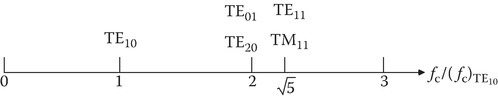
FIGURE 3.3
Normalized cutoff frequencies of a rectangular waveguide with b/a = 1/2.

All other components are zero. The wave impedance in this case is given by

(3.47)

${(Z_{w})}_{{TE}_{10}} = - \frac{{\tilde{E}}_{y}}{{\tilde{H}}_{x}} = \frac{η}{cos ψ},$

where

(3.48)

$cos Ψ = \sqrt{1 - {(\frac{f_{c}}{f})}^{2}} .$

For this case, the cutoff frequency for the TE₁₀ mode is given by

(3.49)

${(f_{c})}_{{TE}_{10}} = \frac{1}{2 a \sqrt{μ ε}} .$

For f > f_c, γ = jβ, where β is real, the mode propagates, and the wave impedance given by Equation 3.47 is real. For f < f_c, γ = α, where α is real, the mode does not propagate, and the wave impedance is imaginary. The electric and the magnetic fields are in time quadrature, and there is no real power flow down the guide. The mode is evanescent and the fields decay signifying localization of stored energy.

3.5Power Flow in a Waveguide: TE₁₀ Mode

It is easy enough to study the power flow of the TE₁₀ mode. From Equation 3.46 and 3.47, we obtain

(3.50)

$〈S_{Z R}〉 = \frac{1}{2} Re [\tilde{E} \times \tilde{H} *] \cdot \hat{z},$

(3.51)

$〈{(S_{Z R})}_{{TE}_{10}}〉 = \frac{1}{2} \frac{η}{cos ψ} {|H_{10}|}^{2} {(\frac{β a}{π})}^{2} {sin}^{2} \frac{π x}{a}, f > f_{c},$

where ψ is as given by Equation 3.48. The power flow P₁₀ is given by

(3.52)

$P_{10} = \int_{0}^{b} \int_{0}^{a} 〈{(S_{Z R})}_{{TE}_{10}}〉 \cdot \hat{z} d x d y = \frac{1}{2} {|H_{10}|}^{2} {(\frac{β a}{π})}^{2} \frac{η}{cos ψ} \frac{a b}{2} .$

3.6Attenuation of TE₁₀ Mode due to Imperfect Conductors and Dielectric Medium

We have seen that the wave attenuates when the signal frequency is less than the cutoff frequency. The wave becomes evanescent. Even if f > f_c, the wave can attenuate due to imperfect materials. The exponential factor of the fields of the wave will have the form

(3.53)

$e^{- γ z} = e^{- (α_{c} + α_{d}) z} e^{- j β z} .$

In the above, α_c is the attenuation of the fields due to the conversion of the wave energy into heat by imperfect conductors of the guide. α_d is the attenuation due to the conversion of the wave energy into heat by an imperfect dielectric. These are given by

(3.54)

$α_{c} = \frac{R_{s} {(Z_{w})}_{{TE}_{10}}}{η^{2} b a} (a + \frac{b λ^{2}}{2 a^{2}}) = \frac{R_{s}}{b η \sqrt{1 - {(\frac{λ}{2 a})}^{2}}} [1 + \frac{2 b}{a} {(\frac{λ}{2 a})}^{2}],$

(3.55)

$α_{d} = \frac{k (\frac{σ}{ω ε})}{2 \sqrt{1 - {(\frac{λ}{2 a})}^{2}}} .$

In the above, R_s is the surface resistance of the conductor and σ/ωε the loss tangent of the dielectric. The derivation of the attenuation constant formulas is given as problems at the end of the book.

3.7Cylindrical Waveguide: TM Modes

Let

(3.56)

${\tilde{E}}_{z} (ρ, ϕ, z) = F (ρ, ϕ) e^{- γ z}$

and

(3.57)

$F (ρ, ϕ) = f_{1} (ρ) f_{2} (ϕ) .$

The separation of variable technique applied to the PDE

(3.58)

$\nabla_{t}^{2} F + k_{c}^{2} F = 0$

results in two ODEs with separation constants k_c and n:

(3.59)

$\frac{1}{ρ} \frac{d}{d ρ} (ρ \frac{d f_{1}}{d ρ}) + (k_{c}^{2} - \frac{n^{2}}{ρ^{2}}) f_{1} = 0,$

(3.60)

$\frac{d^{2} f_{2}}{d ϕ^{2}} + n^{2} f_{2} = 0.$

Recognizing Equation 3.59 as the Bessel equation (2.120), the solution for F may be written as a linear combination of the product of the functions given below:

(3.61)

$F = \{\begin{array}{c} J_{n} (k_{c} ρ) \\ Y_{n} (k_{c} ρ) \end{array}\} \{\begin{array}{c} sin n ϕ \\ cos n ϕ \end{array}\} .$

Since ρ = 0 is a part of the field region, we choose J_n function for the ρ variation and from the boundary condition ${\tilde{E}}_{z} = F = 0$ when ρ = a (see Figure 3.4):

(3.62)

$k_{c} a = χ_{n l},$

where χ_nl is the lth root of J_n and a partial list of these is given in Table 2.4.

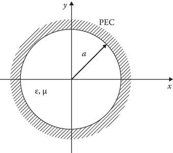
FIGURE 3.4
Circular waveguide with PEC boundary.

The cutoff frequency is given by

(3.63)

${(f_{c})}_{{TM}_{n l}} = \frac{k_{c}}{2 π \sqrt{μ ε}} = \frac{χ_{n l}}{2 π a \sqrt{μ ε}} .$

Since the lowest value for χ_nl is 2.405 when n = 0 and l = 1, the lowest cutoff frequency for TM modes is given by

(3.64)

${(f_{c})}_{{TM}_{01}} = \frac{χ_{01}}{2 π a \sqrt{μ ε}} = \frac{2.405}{2 π a \sqrt{μ ε}} .$

3.8Cylindrical Waveguide: TE Modes

Let

(3.65)

${\tilde{H}}_{z} (ρ, ϕ, z) = G (ρ, ϕ) e^{- γ z} .$

Solution for G is again given by Equation 3.61. However, in the TE case, the Neumann boundary condition

(3.66)

${\frac{\partial G}{\partial ρ} |}_{ρ = a} = 0$

translates into the requirement

(3.67)

$J_{n}^{'} (k_{c} a) = 0,$

where the derivative is with respect to the argument k_cρ. The cutoff wave number is thus given by

(3.68)

${(k_{c})}_{TE} = \frac{χ_{n l}^{'}}{a},$

where $χ_{n l}^{'}$ is the lth root of the derivative of nth-order Bessel function of the first kind. The values of $χ_{n l}^{'}$ are listed in Table 2.4. The lowest value is 1.841 and occurs for n = 1 and l = 1. The lowest cutoff frequency of a circular waveguide is thus given by

(3.69)

${(f_{c})}_{{TE}_{11}} = \frac{1.841}{2 π a \sqrt{μ ε}} .$

3.9Sector Waveguide

Figure 3.5 shows the cross section of a sector waveguide with PEC boundaries.

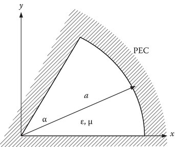
FIGURE 3.5
Sector waveguide with PEC boundaries.

For TM modes, the boundary conditions are the Dirichlet boundary conditions:

(3.70)

$F = 0, ϕ = 0 or α,$

(3.71)

$F = 0, ρ = a .$

From Equation 3.71, the ρ variation is given by the Bessel function of the first kind, however, the order of the Bessel function need not be an integer; the field region in this case is limited to 0 < ϕ < α. In the case of a circular waveguide, the field region is given by 0 < ϕ < 2π. The ϕ variation in such a case is a linear combination of sin nϕ and cos nϕ, where n is an integer. Such stipulation is necessary to ensure a unique value for the potential. Note that cos nϕ and cos n(ϕ + 2π) are equal only if n is an integer. For the sector waveguide, the ϕ variation is again a linear combination of cos νϕ and sin νϕ where ν need not be an integer. Bearing in mind these considerations, we write the potential

(3.72)

$F = J_{ν} (k_{c} ρ) sin ν ϕ,$

where

(3.73)

$ν = \frac{n π}{α} and k_{c} a = χ_{(n π / α) l} .$

For TE modes

(3.74)

$G = J_{ν} (k_{c} ρ) cos ν ϕ,$

where

(3.75)

$k_{c} a = χ_{(n π / α) l}^{'} .$

3.10Dielectric Cylindrical Waveguide: Optical Fiber

We have seen in Sections 3.7 and 3.8 that an electromagnetic wave is guided by a hollow cylindrical tube with a conducting boundary. The fields inside the guide were classified as TM modes (E_z = 0 on the boundary) or TE modes (∂H_z/∂n = 0 on the boundary). In either case, the fields outside the cylinder are zero. Can a cylindrical dielectric rod guide an electromagnetic wave? The answer is yes. A qualitative picture of such wave guiding as a surface wave has been alluded to before in connection with propagation of an electromagnetic wave from an optically dense to optically rare medium when the angle of incidence is greater than the critical angle. In this section, we examine the problem as a boundary value problem. Figure 3.6 shows the variation of the permittivity of a step index optical fiber in its cross section.

In contrast to the conducting guides, one notes here that the boundary condition for this case will be the continuity of the tangential electric and magnetic fields at ρ = a for all ϕ and z:

(3.76)

$E_{z 1} = E_{z 2}, ρ = a,$

(3.77)

$H_{z 1} = H_{z 2}, ρ = a,$

(3.78)

$E_{ϕ 1} = E_{ϕ 2}, ρ = a,$

(3.79)

$H_{ϕ 1} = H_{ϕ 2}, ρ = a .$

This suggests to us that, in general, we may not be able to separate the modes into TE or TM modes. A general mode in this case may be a hybrid mode having E_z and H_z components. However, we can show that the optical fiber guide can have a TM_0l or TE_0l mode of propagation for the special case of n = 0. Let us look at the TM case in detail. Let the ρ variation of E_z be chosen as J₀(k_c1ρ), for 0 < ρ < a and K₀(k_c2ρ) for a < ρ < ∞. The choice of modified Bessel function K₀ in the latter range is to ensure that the amplitude of electromagnetic fields decay as ρ increases. This choice of the admissible function is in contrast to the choice of $H_{0}^{(2)}$ in Equation 2.121 where we needed an outgoing cylindrical wave at ρ = ∞. The formulation is given as follows:

(3.80)

$E_{z 1} = A_{0} J_{0} (k_{c 1} ρ) e^{- j β z}, 0 < ρ < a,$

(3.81)

$E_{z 2} = B_{0} K_{0} (k_{c 2} ρ) e^{- j β z}, a < ρ < \infty,$

where

(3.82)

$k_{c 1}^{2} + β^{2} = k_{1}^{2} = ω^{2} μ_{0} ε_{1},$

(3.83)

$- k_{c 2}^{2} + β^{2} = k_{2}^{2} = ω^{2} μ_{0} ε_{2} .$

It can be shown [1] that the boundary condition (Equations 3.76 and 3.79) can be satisfied if the following transcendental equation is satisfied:

(3.84)

$\frac{J_{1} (k_{c 1} a)}{J_{0} (k_{c 1} a)} = - \frac{ε_{2}}{ε_{1}} \frac{k_{c 1}}{k_{c 2}} \frac{K_{1} (k_{c 2} a)}{K_{0} (k_{c 2} a)} .$

The transcendental equation has several solutions giving rise to several TM modes. Next, let us consider whether the concept of cutoff frequency holds in the dielectric guiding. The cut off occurs when k_c2 = 0, since for negative values of $k_{c 2}^{2}$ , the modified Bessel function K₀ is no longer a monotonic function and the wave in medium 2 is no longer evanescent. Further consideration shows that k_c2 = 0 is equivalent to J₀ (k_c1a) = 0 or

(3.85)

${(k_{c 1})}_{0 l} = \frac{χ_{0 l}}{a}$

and

(3.86)

${(k_{c 1})}_{01} = \frac{χ_{01}}{a} = \frac{2.4049}{a} .$

Note that at cutoff

(3.87)

$k_{c 1}^{2} = k_{1}^{2} - β^{2} = k_{1}^{2} - (k_{2}^{2} + k_{c 2}^{2}) = k_{1}^{2} - k_{2}^{2} .$

For TE_0l modes, the eigenvalue equation is given by

(3.88)

$\frac{J_{1} (k_{c 1} a)}{J_{0} (k_{c 1} a)} = - \frac{k_{c 1}}{k_{c 2}} \frac{K_{1} (k_{c 2} a)}{K_{0} (k_{c 2} a)} .$

If n ≠ 0, then the fields do not separate into TE and TM modes. All the fields become coupled through the continuity conditions. The modes are hybrid and have both E_z and H_z nonzero. The fields for the two regions may be written as [1]

(3.89)

$\begin{array}{l} ρ < a, \\ E_{z 1} = A J_{n} (u \frac{ρ}{a}) {\begin{matrix} \cos n ϕ \\ \sin n ϕ \end{matrix}}, \\ H_{z 1} = B J_{n} (u \frac{ρ}{a}) {\begin{matrix} \cos n ϕ \\ \sin n ϕ \end{matrix}}, \\ u^{2} = (k_{1}^{2} - β^{2}) a^{2}, \end{array} \begin{array}{l} ρ > a \\ E_{z 2} = C K_{n} (w \frac{ρ}{a}) {\begin{matrix} \cos n ϕ \\ \sin n ϕ \end{matrix}} \\ H_{z 2} = D K_{n} (w \frac{ρ}{a}) {\begin{matrix} \cos n ϕ \\ \sin n ϕ \end{matrix}} \\ w^{2} = (β^{2} - k_{2}^{2}) a^{2}, \end{array}$

The transverse components may be obtained from Maxwell’s equations. Applying the boundary conditions (Equation 3.76, Equation 3.77, Equation 3.78 and Equation 3.79), one can obtain the eigenvalue equation [1]

(3.90)

${[\frac{k_{1} J_{n}^{'} (u)}{u J_{n} (u)}]}^{2} + {[\frac{k_{2} K_{n}^{'} (u)}{w K_{n} (u)}]}^{2} + \frac{k_{1}^{2} + k_{2}^{2}}{u w} [\frac{J_{n}^{'} (u) K_{n}^{'} (w)}{J_{n} (u) K_{n} (w)}] = \frac{β^{2} n^{2} v^{4}}{u^{4} w^{4}},$

where

(3.91)

$v^{2} = u^{2} + w^{2} = (k_{1}^{2} - k_{2}^{2}) a^{2} .$

The solutions of the transcendental equation (3.90) may be designated as χ_nl. For n ≠ 0, we get hybrid modes designated as HEM (hybrid electric and magnetic). The HEM modes with odd values of the second subscript are called HE modes, whereas HEM modes with even values for the second subscript are called EH modes. HE₁₁ mode has no cutoff frequency and so is often called the dominant mode. From [2] and [3], a plot of β/k₀ versus 2a/λ₀ for HE₁₁ mode, TE₀₁ mode, and TM₀₁ mode for the case of ε_r1 = 2.56, ε_r2 = 1, k₂ = k₀, λ₀ = 2π/k₀ is obtained (see Figure 3.7). For $2 a / λ_{0} < 2.4049 / π \sqrt{ε_{r} - 1}$ , only the dominant HE₁₁ mode exists.

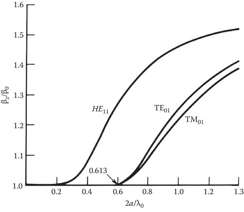
FIGURE 3.7
Ratio of β/k₀ for the first three surface-wave modes on a polystyrene rod (ε_r = 2.26). (Adapted from Collin, R.E., *Field Theory of Guided Waves*, McGraw-Hill, New York, 1960 [3].)

References

1.Ramo, S., Whinnery, J.R., and Van Duzer, T. V., Fields and Waves in Communication Electronics, 3rd edn., Wiley, New York, 1994.
2.Balanis, C.A., Advanced Engineering Electromagnetics, Wiley, New York, 1989.
3.Collin, R.E., Field Theory of Guided Waves, McGraw-Hill, New York, 1960.

..................Content has been hidden....................

You can't read the all page of ebook, please click here login for view all page.

Table of Contents for 3. Two-Dimensional Problems and Waveguides

Create new playlist

Sign In

Sign Up

Table of Contents for
3. Two-Dimensional Problems and Waveguides