
]>
Appendix 14C: Reflection and Transmission of Electromagnetic Waves Obliquely Incident on a Relativistically Moving Uniaxial Plasma Slab*
14C.1Introduction
The electromagnetic wave interaction with relativistic plasmas has been receiving considerable attention in recent literature. A number of investigators [1,2,3,4,5,6,7,8,9,10,11,12,13,14] have studied the problem of reflection and transmission of electromagnetic waves by semi-infinite moving dielectric media and plasmas as well as dielectric slabs. Yeh [15,16] studied the reflection and transmission of electromagnetic waves by a moving isotropic plasma slab, whereas Chawla and Unz [17] considered the case of normal incidence on a moving plasma slab subjected to a finite static magnetic field normal to the slab. Kong and Cheng [18] obtained numerical results for the transmission coefficient at normal incidence when the uniaxial plasma slab is moving along the interface and the technique used was based on the concept of bianisotropy.
The purpose of this appendix is to present the solution for reflection and transmission coefficients of parallel-polarized electromagnetic waves incident on a relativistically moving anisotropic plasma slab with strong normal magnetostatic field. The emphasis is on the nature of oscillations in the reflection and transmission coefficients (due to the interference of internally reflected waves) that are discussed against the incident wave frequency as well as the velocity of the slab, the latter being the more interesting one.
The problem is solved in the rest system of the slab and relativistic transformations are then used to obtain the reflection and transmission coefficients as observed in the laboratory system.
14C.2Formulation of Problem
The geometry of the problem is shown in Figure 14C.1. Consider a plane wave excited in the laboratory system Σ propagating in free space in the xz-plane at an angle θ to the positive z-axis. Assuming a harmonic time variation the wave takes the form
where kx = k0 sin θ = k0S, kz = k0 cos θ = k0C, k0 = ω/c, and c=1/(μ0ϵ0)1/2
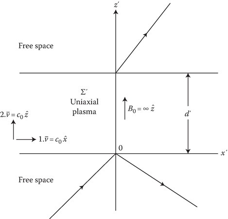
FIGURE 14C.1
Geometry of the problem. (Reprinted from Kalluri, D. and Shrivastava, R.K., Reflection and transmission of electromagnetic waves obliquely incident on a relativistically moving uniaxial plasma slab, IEEE Trans. Antennas Propagat., AP-21, 63–70. © 1973 IEEE. With permission.)
This wave is transformed to the Σ′ system that is stationary with respect to the moving plasma slab bounded by the planes z′ = 0 and z′ = d′. The infinitely strong magnetostatic field is assumed to be normal to the slab, so that the plasma medium may be modeled as a uniaxially anisotropic dielectric medium whose relative dielectric constant is a tensor:
where ωp is the plasma frequency and ω′ the wave frequency in the Σ′ system.
In the moving system Σ′, the exponential variation of the field components takes the form
where k′x=k′0S′
The reflected and transmitted waves, respectively, must then have the following exponential variation:
In the stationary system Σ, the corresponding forms for the reflected and transmitted waves are
Using Maxwell’s equations in free space, one can obtain all other field components:
in the Σ′ system, and
in the Σ system.
Making use of the principle of phase invariance of the plane waves, the covariance of Maxwell’s equations, and the Lorentz transformations, one obtains the following relations between the primed and unprimed quantities [4,11,19] for the two cases of slab motion.
Case 1: ˉυ=υ0ˆx.
υ¯=υ0xˆ. (14C.10a)ω′=pxω,k′x=γk0(S−β),k′z=k0C,ω′=pxω,k′x=γk0(S−β),k′z=k0C, (14C.10b)ωr=ωt=ω,krx=ktx=k0S,krz=ktz=k0C,ωr=ωt=ω,krx=ktx=k0S,krz=ktz=k0C, (14C.10c)C′=Cpx,S′=S−β1−Sβ,E′I,T,Rx=EI,T,Rx,C′=Cpx,S′=S−β1−Sβ,E′I,T,Rx=EI,T,Rx, where
(14C.10d)β=υ0c,γ=1(1−β2)1/2andpx=g(1−Sβ).β=υ0c,γ=1(1−β2)1/2andpx=g(1−Sβ). Case 2: ˉυ=υ0ˆz
υ¯=υ0zˆ .(14C.11a)ω′=pzω,k′x=k0S,k′z=γk0(C−β),ω′=pzω,k′x=k0S,k′z=γk0(C−β), (14C.11b)ωr=γ2ω(1+β2−2βC)krz=k0S,krz=γ2k0[(1+β2)C−2β],ωr=γ2ω(1+β2−2βC)krz=k0S,krz=γ2k0[(1+β2)C−2β], (14C.11c)ωt=ω,ktx=k0S,ktz=k0C,ωt=ω,ktx=k0S,ktz=k0C, (14C.11d)C=C−β1−Cβ,S=Spz,C=C−β1−Cβ,S=Spz, (14C.11e)E′I,Tx=γ(1−βC)EI,Tx,E′Rx=γ(1−ββ′C)ERx,E′I,Tx=γ(1−βC)EI,Tx,E′Rx=γ(1−ββ′C)ERx, where
(14C.11f)pz=γ(1−Cβ)andβ′=1+β2−2βC1+β2−2β/C.pz=γ(1−Cβ)andβ′=1+β2−2βC1+β2−2β/C.
It can easily be seen that
where θr is the angle of reflection as seen from the Σ system.
14C.3Dispersion Relation and Other Relations
Let the waves in the plasma have the exponential variation:
Using Maxwell’s equations in the plasma, one obtains
On substituting for S′ and єz from Equations 14C.2, 14C.10, and 14C.11, the dispersion coefficient q′ relevant to the two cases of slab motion may be written as
and
Ω(= ω/ωp) being the normalized incident wave frequency.
14C.4Reflection and Transmission Coefficients
Making use of the usual continuity conditions of tangential electromagnetic fields at the boundaries z′ = 0 and z′ = d′ in the rest frame Σ′ of the plasma and then transforming the field strengths in the observer’s frame Σ according to Equations 14C.10c and 14C.11e, one can derive the expressions for the power reflection and transmission coefficients (ρ and τ, respectively) as observed in the Σ frame.
Case 1: ˉυ=υ0ˆx
υ¯=υ0xˆ .(14C.15a)ρx=|ERxEIx|2=11+[2q′xC′/(q′2x−C′2)coseck′0q′xd′]2,ρx=∣∣∣ERxEIx∣∣∣2=11+[2q′xC′/(q′2x−C′2)coseck′0q′xd′]2, (14C.15b)τx=|ETxEIx|2=11+[((q′2x−C′2)/2q′xC′)sink′0q′xd′]2.τx=∣∣∣ETxEIx∣∣∣2=11+[((q′2x−C′2)/2q′xC′)sink′0q′xd′]2. Case 2: ˉυ=υ0ˆz
υ¯=υ0zˆ .(14C.16a)ρz=β′|ERxEIx|2=β′|C−βC+ββ′|211+[(2q′zC′/(q′2z−C′2))coseck′0q′zd′]2,ρz=β′∣∣∣ERxEIx∣∣∣2=β′∣∣∣C−βC+ββ′∣∣∣211+[(2q′zC′/(q′2z−C′2))coseck′0q′zd′]2, (14C.16b)τz=|ETxEIx|2=11+[((q′2z−C′2)/2q′zC′)sink′0q′zd′]2.τz=∣∣∣ETxEIx∣∣∣2=11+[((q′2z−C′2)/2q′zC′)sink′0q′zd′]2.
14C.5Numerical Results and Discussion
Substituting for q′, the reflection and transmission coefficients take the form
in the real range of q′ and
in the imaginary range of q′, where α, A, and B for the two cases of slab motion are given by the following.
Case 1:
(14C.18a)αx=1αx=1 (14C.18b)Ax=2πΩpx(C2Ω2−1p2xΩ2−1)1/2⋅d′p,Ax=2πΩpx(C2Ω2−1p2xΩ2−1)1/2⋅d′p, (14C.18c)Bx=4p2xC2(p2xΩ2−1)(C2Ω2−1)(p2x−C2)2.Case 2:
(14C.19a)αz=(1+β2−2βC)(1+β2−2β/C)(1−β2)2,(14C.19b)Az=2πΩpz((p2z−S2)Ω2−1p2zΩ2−1)1/2⋅d′p,(14C.19c)Bz=4p2z(p2z−S2)(p2zΩ2−1)[(p2z−S2)Ω2−1]S4,
where d′p=d′/λp, λp being the free-space wavelength corresponding to the plasma frequency.
It is thus seen that ρ is an oscillatory function in the real range of q′, whereas for imaginary q′ it is nonoscillatory. The reflection coefficient is now discussed as a function of the normalized wave frequency (Ω) and the slab velocity (β).
14C.5.1Variation with Ω
Numerical results were obtained for C = 0.5, dp′ = 1, and p = 1.1. Figures 14C.2 and 14C.3 show the plot of q′ and ρ versus Ω for the two cases of slab motion. For obtaining the maxima and minima in the oscillatory ranges [20], it should be noted that ρmin is zero and this occurs for Ω satisfying the equation

FIGURE 14C.2
Characteristic root (q′x) and power reflection coefficient (ρx) as functions of normalized wave frequency for slab motion parallel to the interface. Dashed portion of the curve indicates imaginary values of q′x. (Reprinted from Kalluri, D. and Shrivastava, R.K., Reflection and transmission of electromagnetic waves obliquely incident on a relativistically moving uniaxial plasma slab, IEEE Trans. Antennas Propagat., AP-21, 63–70. © 1973 IEEE. With permission.)
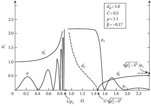
FIGURE 14C.3
Characteristic root (q′z) and power reflection coefficient (ρz) as functions of normalized wave frequency for slab motion normal to the interface. Dashed portion of the curve indicates imaginary values of q′z. (Reprinted from Kalluri, D. and Shrivastava, R.K., Reflection and transmission of electromagnetic waves obliquely incident on a relativistically moving uniaxial plasma slab, IEEE Trans. Antennas Propagat., AP-21, 63–70. © 1973 IEEE. With permission.)
This is equivalent to the condition 2q′d′ = (n/2)λ′ (n even), which means that the optical path difference between two successive reflected waves (there being an infinite series of internal reflections inside the plasma layer) is an integral multiple of one wavelength, so that these waves have the same phase and reinforce each other and in this case the first reflected wave from the lower boundary exactly annuls the resultant of the remaining reflected waves, thus giving zero reflection [21].
Thus, one obtains, after some algebra,
and
The minus sign in the preceding equations gives the minima in the first oscillatory range, while the plus sign in the other range. There are thus an infinite number of oscillations in either range.
The maxima in ρ occur for Ω satisfying the transcendental equation
where
and
The maximum point between the two minima of a loop was first determined using a subroutine to solve the preceding transcendental equation. Having located this maximum, each interval between the minimum and ρ maximum points was divided into a number of parts and calculated at each point. This procedure was repeated to get the second loop and so on.
It is seen from the curves in Figures 14C.2 and 14C.3 that as q′ tends to infinity in its real range, the oscillations in ρ become more and more rapid and of increasing amplitude. In the other range (where q′ reaches its asymptotic limit C′), the oscillations slow down progressively as Ω is increased and ultimately die down. The rapidity of oscillations is due to steep rise in q′ with Ω in this range. The amplitude of oscillations is governed by the magnitude of q′. This is easily seen by noting that if we ignore the oscillations and draw a curve representing average value, this will give the ρ versus Ω curve for the semiinfinite case. For this case, reflection will be strong when the free-space fields are badly matched [22] to the plasma fields (q′ ≠ C′) and zero when the free-space fields are perfectly matched to the plasma fields (q′ = C′).
As is known, ρ + τ > 1 and the reflected wave emerges out amplified when the slab moves toward the incident wave. This is because the stored energy decreases and mechanical power has to be externally supplied to the medium against the radiation pressure exerted by the field on the medium. When the medium has a tangential velocity, the force on its surface can do no work and the time-averaged stored energy remains constant, thus giving ρ + τ = 1 for parallel motion [11].
14C.5.2Variation with β
It will be seen from the equations that the reflection and transmission coefficients are complicated functions of the slab velocity. To study these coefficients directly against β would be too involved. So, the following technique is evolved.
q′ is first studied against p and ρ/α plotted against p, since the maxima and minima of this curve are easily obtained as before.
p is studied against β. The parameter p (= ω′/ω) is significant in that it transforms the incident wave frequency to the rest system of the plasma. It is a quadratic in β and the two values of β for any p are given by
(14C.22a)(β1,2)x=Sp2x+S2±[(Sp2x+S2)2+p2x−1p2x+S2]1/2and
(14C.22b)(β1,2)z=Cp2z+C2±[(Cp2z+C2)2+p2z−1p2z+C2]1/2.The plot of p versus β for C = 0.5 is given in Figure 14C.4. It shows the variation of ω′ with β.
ρ/α is now plotted against β by combining the preceding two steps. With reference to a different horizontal axis (ρ/α = 1), this represents τ.
α versus β is studied according to Equation 14C.19a and plotted for C = 0.5 along with the ρ/α versus β curve.
Finally, ρ is obtained as a function of β using steps 3 and 4.
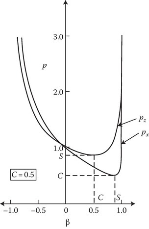
FIGURE 14C.4
Parameter p as a function of the normalized slab velocity (β = v0/c). p being ω′/ω, the curve shows variation of ω′ with β. The subscripts x and z on p indicate the direction of slab motion. (Reprinted from Kalluri, D. and Shrivastava, R.K., Reflection and transmission of electromagnetic waves obliquely incident on a relativistically moving uniaxial plasma slab, IEEE Trans. Antennas Propagat., AP-21, 63–70. © 1973 IEEE. With permission.)
It should be noted that since α = 1 for parallel slab motion, the development of the ρ versus β curve in this case involves only three steps, q′ versus p gives interesting results. q′ is seen to vary in a different manner with p for various ranges of Ω given by Ω < 1/C, Ω = 1/C, and Ω > 1/C for slab motion parallel to the interface and Ω ≤ 1/S and Ω > 1/S for normal motion.
14C.5.3Slab Motion Parallel to Interface (ˉυ=υ0ˆx)
Numerical results were obtained for C = 0.5, d′p=1 in the three ranges of values of aforementioned Ω. For Ω = 1/C, q′ = 0 and it can be shown that ρx for this case is given by
For the other two cases, namely Ω < 1/C and Ω > 1/C, curves were obtained with Ω = 1.2 and 2.5, respectively (1/C = 2).
The plot of q′x and ρx against px has been shown in Figure 14C.5 (for Ω < 1/C). In the oscillatory range, (ρmin)x is zero and occurs for px given by
Thus, one obtains
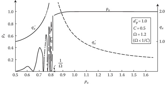
FIGURE 14C.5
q′x and ρx versus px, for Ω > 1/C, slab motion being parallel to the interface. Dashed portion of the curve indicates imaginary values of q′x. (Reprinted from Kalluri, D. and Shrivastava, R.K., Reflection and transmission of electromagnetic waves obliquely incident on a relativistically moving uniaxial plasma slab, IEEE Trans. Antennas Propagat., AP-21, 63–70. © 1973 IEEE. With permission.)
It should also be noted that there is an additional minimum point at px = C. This is readily seen by setting Bx = α in Equation 14C.18c. For this condition, q′ = C′ = 1 representing a perfect match for the free-space and plasma fields and the incident wave is wholly transmitted.
The maxima in ρx occur for px satisfying the transcendental equation tan Ax = (fp)xAx, where
Case 1: Ω < 1/C.
It should be noted in Equation 14C.23 that n = 0 is not a permissible even integer since this will correspond to a zero value of px. The lowest permissible even integer may be determined from the minimum value of px that equals C. This value of px corresponds to n = n′ = 4dpΩC. Since this value may not be an even integer, the lowest permissible even integer is the one that is greater than n′. The highest permissible value for n is infinity when px = 1/Ω. Beyond the oscillatory region, ρx is monotonic.
The ρx versus px curve is finally developed into the ρx versus β curve (Figure 14C.6) with the help of px versus β curve that has been earlier explained. As there are two values of β for any px, one loop in the ρx versus px curve leads to two loops in the ρx versus β curve, the two loops being one on each side of β = S (corresponding to the starting point px = C in the ρx versus px curve).
It is seen from the curve that ρx is oscillatory in the range of β from 0.23 to 0.98 and for other values of β, ρx is monotonic. The rapidity of the oscillations (of increasing amplitude) increases as one approaches the end of the oscillatory region on both sides of β = S. The oscillations are even more rapid to the right of β = S than to the left. This is because the wavelength λ′ decreases much faster in the right range than the left range as can be seen from an inspection of the px versus β curve.
Case 2: Ω > 1/C
Referring to Equation 14C.23 again, it should be noted that n cannot assume all even integer values. The limits on n are set from the requirement that pmin has to lie between C and ∞. px = C corresponds to n = n′ = 4dp′ΩC and px = ∞ corresponds to
Noting that n″ < n′, the lowest permissible value for n is an even integer which is greater than or equal to n″. The highest permissible value of n is again an even integer that is less than or equal to n′.
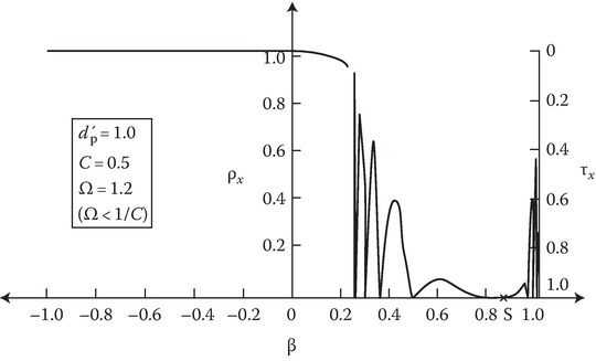
FIGURE 14C.6
ρx and τx versus β, for Ω > 1/C, slab motion being parallel to the interface. (Reprinted from Kalluri, D. and Shrivastava, R.K., Reflection and transmission of electromagnetic waves obliquely incident on a relativistically moving uniaxial plasma slab, IEEE Trans. Antennas Propagat., AP-21, 63–70. © 1973 IEEE. With permission.)
For the chosen data of d′p = 1, C = 0.5, and Ω = 2.5, range of n as given by Equation 14C.25 is 3–5 and as only even n is allowed, the value to be used is 4. This corresponds to px = 0.6. Thus, we have only two minima in ρx, one at px = 0.5 and the other at px = 0.6, giving one loop in the region.
For any other data, the number of the oscillatory loops will change. For example, if dp′ = 10, C = 0.5, and Ω = 2.1, we have n′ = 42 and n″ = 12.8. So n″ has to be taken as 14 (the next higher even number), giving the range of n as 14–42. This leads to 14 oscillatory loops and as n = 14 corresponds to px = 1.18, it will be seen that all these loops will be in the range of px from 0.5 to 1.18, which means intense crowding of the oscillations in the region.
As px tends to infinity, Ax tends to 2πd′p(Ω2C2−1)1/2 and Bx tends to 4Ω2C2(Ω2C2 – 1) (refer Equation 14C.18). Thus, as px increases beyond the oscillatory region, ρx rises asymptotically to a value given by
and
Only the final plot of ρx versus β is shown (Figure 14C.7), from which it is seen that after some oscillation, the reflection coefficient increases to its final value on either side of β = S, the rise to the right of β = S being extremely steep when compared to the slow rise in the left region. A physical explanation has already been given.
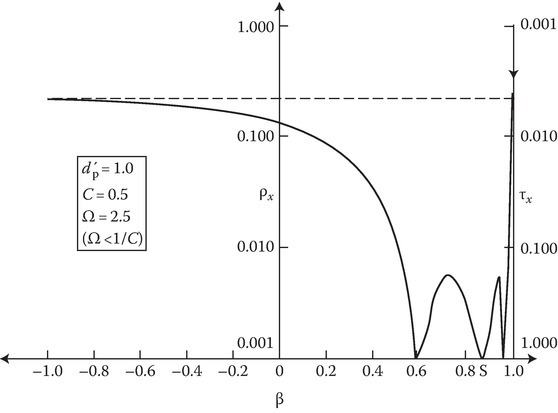
FIGURE 14C.7
ρx and τx versus β, for Ω > 1/C, slab motion being parallel to the interface. (Reprinted from Kalluri, D. and Shrivastava, R.K., Reflection and transmission of electromagnetic waves obliquely incident on a relativistically moving uniaxial plasma slab, IEEE Trans. Antennas Propagat., AP-21, 63–70. © 1973 IEEE. With permission.)
14C.5.4Slab Motion Normal to Interface (ˉυ=υ0ˆz)
Curves were obtained for Ω = 0.5 (<1/S) and Ω = 2.0 (>1/S) taking d′p = 1 and C = 0.5. Figures 14C.8 and 14C.11 show the plot of qz and ρz/αz versus pz for the two ranges of Ω. The maxima and minima in ρz/αz are obtained as before and occur for pz given by
(the minus sign before the square-root sign is not permissible for Ω > 1/S as in this case q′z is real in one range only, that is, [S2 + (1/Ω2)]1/2 < pz < ∞) and tan Az = (fp)zAz, where
Case 1: Ω < 1/S.
The minimum value of pz is S and this corresponds to n = n′ = 4dp′ΩS/(1 – Ω2S2)1/2. Since this value may not be an even integer, the lowest permissible even integer is the one that is greater than n′. The highest permissible value of n is, of course, infinity corresponding to pz = 1/Ω.
The development of the ρz versus β curve is illustrated in Figure 14C.8, Figure 14C.9 and Figure 14C.10 following the procedure described before. The significant point to be noted here is the appearance of an additional factor αz in the expression for reflection coefficient. This is actually the reflection coefficient for a perfect moving minor [11] and the multiplier 1/(1 + Bz cosec2 Az) is because of the uniaxial anisotropy of the slab.
It is seen (Figure 14C.9) that starting from infinity αz reduces to unity as β varies from −1 to 0. Thus the reflected wave emerges out amplified in this range (physical explanation given before). In the range 0 < β < (1 − S)/C, αz reduces from 1 to 0. So, the reflection coefficient is less than unity in the above range, finally becoming zero at β = (1 – S)/C. In this range, the energy balance may be shown as
Thus, when the medium recedes from the incident wave, field supplies work to the medium. At β = (1 – S)/C, the angle of reflection θR = 90°, thus explaining the zero-reflected power (Figure 14C.11).
Oscillations in the reflection coefficient have been explained before.
Case 2: Ω ≥ 1/S.
ρz versus β is shown in Figure 14C.12 for Ω = 2.0 (>1/S) taking d′p = 1 and C = 0.5. This may be compared with the previous curve for Ω < 1/S (Figure 14C.10) noting that the difference is because of just one oscillatory range for ρz in the former in contrast to the two oscillatory ranges in the latter.
The curve for Ω = 1/S is similar to the preceding and hence not given.
At β greater than or equal to C, the incident wave from below (Figure 14C.1) has no interaction with the slab since the normal component of the phase velocity of the wave is less than or equal to that of the slab. However, the results given here are applicable even when β > C if the problem is understood to be that the slab impinges on the portion of an existing incident wave above the slab. This aspect of the problem will be reported later.

FIGURE 14C.8
q′z and ρz/αz versus pz, for Ω < 1/S, normal slab motion. Dashed portion of the curve indicates imaginary values of q′z. (Reprinted from Kalluri, D. and Shrivastava, R.K., Reflection and transmission of electromagnetic waves obliquely incident on a relativistically moving uniaxial plasma slab, IEEE Trans. Antennas Propagat., AP-21, 63–70. © 1973 IEEE. With permission.)
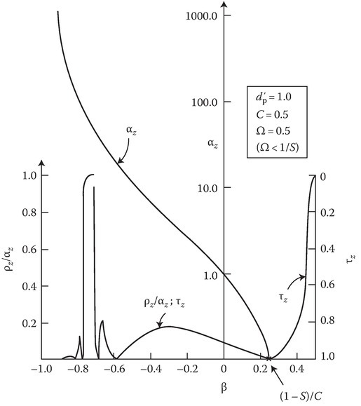
FIGURE 14C.9
ρz/αz and τz as functions of β, for Ω < 1/S, normal slab motion. The curve αz versus β is also shown. (Reprinted from Kalluri, D. and Shrivastava, R.K., Reflection and transmission of electromagnetic waves obliquely incident on a relativistically moving uniaxial plasma slab, IEEE Trans. Antennas Propagat., AP-21, 63–70. © 1973 IEEE. With permission.)
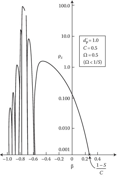
FIGURE 14C.10
ρz versus β, for Ω < 1/S, normal slab motion. (Reprinted from Kalluri, D. and Shrivastava, R.K., Reflection and transmission of electromagnetic waves obliquely incident on a relativistically moving uniaxial plasma slab, IEEE Trans. Antennas Propagat., AP-21, 63–70. © 1973 IEEE. With permission.)

FIGURE 14C.11
q′z and ρz/αz versus pz, for Ω > 1/S, normal slab motion. (Reprinted from Kalluri, D. and Shrivastava, R.K., Reflection and transmission of electromagnetic waves obliquely incident on a relativistically moving uniaxial plasma slab, IEEE Trans. Antennas Propagat., AP-21, 63–70. © 1973 IEEE. With permission.)
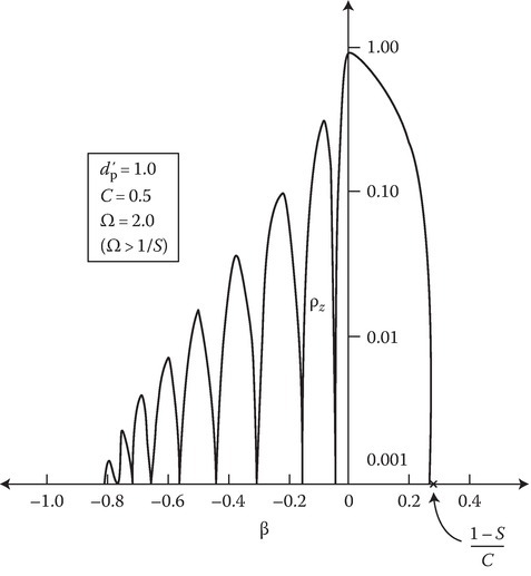
FIGURE 14C.12
ρz versus β, for Ω > 1/S, normal slab motion. (Reprinted from Kalluri, D. and Shrivastava, R.K., Reflection and transmission of electromagnetic waves obliquely incident on a relativistically moving uniaxial plasma slab, IEEE Trans. Antennas Propagat., AP-21, 63–70. © 1973 IEEE. With permission [23].)
References
- 1.Landecker, K., Possibility of frequency multiplication and wave amplification by means of some relativistic effect, Phys. Rev., 86, 449–455, 1952.
- 2.Tai, C. T., Two scattering problems involving moving media, Antenna Lab., Ohio State Univ., Columbus, OH, Rep. 1691–1697, 1964.
- 3.Yeh, C., Reflection and transmission of electromagnetic waves by a moving dielectric medium, J. Appl. Phys., 36, 3513–3517, 1965.
- 4.Yeh, C. and Casey, K. F., Reflection and transmission of electromagnetic waves by a moving dielectric slab, Phys. Rev., 144, 665–669, 1966.
- 5.Yeh, C., Brewster angle for a dielectric medium moving at relativistic speed, J. Appl. Phys., 38, 5194–5200, 1967.
- 6.Yeh, C., Reflection and transmission of electromagnetic waves by a moving dielectric slab II. Parallel polarisation, Phys. Rev., 167, 875–877, 1968.
- 7.Pyati, V. P., Reflection and transmission of electromagnetic waves by a moving dielectric medium, J. Appl. Phys., 38, 652–655, 1967.
- 8.Lee, S. W. and Lo, Y. T., Reflection and transmission of electromagnetic waves by a moving uniaxially anisotropic medium, J. Appl. Phys., 38, 870–875, 1967.
- 9.Tsai, C. S. and Auld, B. A., Wave interaction with moving boundaries, J. Appl. Phys., 38, 2106–2115, 1967.
- 10.Shiozawa, T., Hazama, K., and Kumagai, N., Reflection and transmission of electromagnetic waves by a dielectric half-space moving perpendicular to the plane of incidence, J. Appl. Phys., 38, 4459–4461, 1967.
- 11.Daly, P. and Gruenberg, H., Energy relations for plane waves reflected from moving media, J. Appl. Phys., 38, 4486–4489, 1967.
- 12.Shiozawa, T. and Kumagai, N., Total reflection at the interface between relatively moving media, Proc. IEEE, 55, 1243–1244, 1967.
- 13.Kong, J. A. and Cheng, D. K., Wave behavior at an interface of a semi-infinite moving anisotropic medium, J. Appl. Phys., 39, 2282–2286, 1968.
- 14.Cheng, D. K. and Kong, J. A., Time-harmonic fields in source-free bi-anisotropic media, J. Appl. Phys., 39, 5792–5796, 1968.
- 15.Yeh, C., Reflection and transmission of electromagnetic waves by a moving plasma medium, J. Appl. Phys., 37, 3079–3082, July 1966.
- 16.Yeh, C., Reflection and transmission of electromagnetic waves by moving plasma medium, II. Parallel Polarization, J. Appl. Phys., 38, 2871–2873, 1967.
- 17.Chawla, B. R. and Unz, H., Reflection and transmission of electromagnetic waves normally incident on a plasma slab moving uniformly along a magnetostatic field, IEEE Trans. Antennas Propagat., AP-17, 771–777, 1969.
- 18.Kong, J. A. and Cheng, D. K., Reflection and transmission of electromagnetic waves by a moving uniaxially anisotropic slab, J. Appl. Phys., 40, 2206–2212, 1969.
- 19.Chawla, B. R. and Unz, H., Electromagnetic Waves in Moving Magneto-Plasmas, Kansas University Press, Lawrence, KS, 1971.
- 20.Kalluri, D. and Prasad, R. C., Thin film reflection properties of isotropic and uniaxial plasma slabs, Appl. Sci. Res., 27, 415–424, 1973.
- 21.Budden, K. G., Radio Waves in the Ionosphere, Cambridge University Press, Cambridge, U.K., p. 111, 1961.
- 22.French, I. P., Cloutier, G. G., and Bachynski, M. P., The absorptivity spectrum of a uniform anisotropic plasma slab, Can. J. Phys., 39, 1273–1290, 1961.
- 23. Kalluri, D. and Shrivastava, R. K., Reflection and transmission of electromagnetic waves obliquely incident on a relativistically moving uniaxial plasma slab, IEEE Trans. Antennas Propagat., AP-21, 63–70, 1973.