Search in book...
Toggle Font Controls
Create new playlist

Name your new playlist

Playlist description (optional)
Sign In

Email address

Password

Forgot Password?

or

Continue with Facebook

Continue with Google
Sign Up

Full Name

Email address

Confirm Email Address

Password

or

Continue with Facebook

Continue with Google

Appendix 10C: Waveguide Modes of a Warm Drifting Uniaxial Electron Plasma*

Appendix 10C: Waveguide Modes of a Warm Drifting Uniaxial Electron Plasma *

Dikshitulu K. Kalluri

10C.1Introduction

The guided wave propagation in an anisotropic plasma medium is investigated by many authors. The results for a cold stationary anisotropic plasma are well summarized by Allis et al. [1]. The guided slow-wave propagation in drifting cold anisotropic plasma is considered by Trivelpiece [2]. Mode theory of a waveguide filled with stationary warm uniaxial plasma has been recently reported by Tuan [3]. Electron stream interactions with a cold plasma in a waveguide are considered by Smullin and Chorney [4] and Briggs [5].

In this appendix, the guided wave propagation in a drifting warm plasma in an infinite static magnetic field is investigated with emphasis on the phase characteristics of the waves. The motivation for such a study was provided by an investigation by Articolo [6] on modeling the drifting warm anisotropic plasma medium as a dielectric medium with temporal and spatial dispersions under the assumptions that (1) the neutral molecules and positive ions are cold, (2) the electrons are warm with an average temperature and have a preferred drift superimposed on their thermal motion, and (3) the drift and thermal velocities are nonrelativistic. The additional assumptions made here are that (1) the drift velocity υ₀ is along the z-axis, (2) the static magnetic field of infinite strength is also along the z-axis, and (3) collisional effects are neglected.

10C.2Basic Equations

Let all field quantities vary as

(10C.1)

F_{1} (x, y, z, t) = F (x, y) e^{j w t - γ z} .

$F_{1} (x, y, z, t) = F (x, y) e^{j w t - γ z} .$

The Maxwell equations are

(10C.2)

\bar{\nabla} \times \bar{H} = j ω ε_{0} \bar{ε} \cdot \bar{E},

$\bar{\nabla} \times \bar{H} = j ω ε_{0} \bar{ε} \cdot \bar{E},$

(10C.3)

\bar{\nabla} \times \bar{H} = - j ω μ_{0} \bar{H} .

$\bar{\nabla} \times \bar{H} = - j ω μ_{0} \bar{H} .$

For the case of an infinite static magnetic field and the drift velocity υ₀ both lying along the positive z-axis, it can be shown [6] that

(10C.4)

\bar{ε} (ω, γ) = ​ \hat{x} \hat{x} ​ + \hat{y} \hat{y} ​ + ε_{3} \hat{z} \hat{z},

$\bar{ε} (ω, γ) = \hat{x} \hat{x} + \hat{y} \hat{y} + ε_{3} \hat{z} \hat{z},$

(10C.5)

ε_{3} (ω, γ) = 1 - \frac{ω_{p}^{2}}{{(ω + j γ v_{0})}^{2} + a^{2} γ^{2}},

$ε_{3} (ω, γ) = 1 - \frac{ω_{p}^{2}}{{(ω + j γ v_{0})}^{2} + a^{2} γ^{2}},$

where a is the acoustic velocity indicative of the average temperature of the plasma and ω_p the plasma frequency. From Equation 10C.1, Equation 10C.2 and Equation 10C.3, the expressions for the transverse field ${\bar{E}}_{t} and {\bar{H}}_{t}$ ${\bar{E}}_{t} and {\bar{H}}_{t}$ in terms of E_z and H_z and the wave equations for H_z can be derived. These are the same as for the stationary case derived by Tuan [3] and need not be repeated here. From the wave equation for H_z, it may also be concluded that the TE modes are unaffected by the presence of the plasma.

From the wave equation for E_z, we have

(10C.6)

[\nabla_{t}^{2} + (γ^{2} + k_{0}^{2}) ε_{3}] E_{z} = 0,

$[\nabla_{t}^{2} + (γ^{2} + k_{0}^{2}) ε_{3}] E_{z} = 0,$

where $k_{0}^{2} = ω^{2} μ_{0} ε_{0}$ $k_{0}^{2} = ω^{2} μ_{0} ε_{0}$ and ∇_t is the transverse part of the ∇ operator. The dispersion relation for TM modes can be shown to be

(10C.7)

(γ^{2} + k_{0}^{2}) ε_{3} = {(\frac{ω_{c}}{c})}^{2},

$(γ^{2} + k_{0}^{2}) ε_{3} = {(\frac{ω_{c}}{c})}^{2},$

where ω_c is the cutoff frequency of the empty waveguide and c is the velocity of light. Letting γ = jβ, where β is the propagation constant, Equation 10C.7 may be written as

(10C.8)

(ω^{2} - β^{2} c^{2}) [1 - \frac{ω_{p}^{2}}{{(ω - v_{0} β)}^{2} - a^{2} β^{2}}] = ω_{c}^{2} .

$(ω^{2} - β^{2} c^{2}) [1 - \frac{ω_{p}^{2}}{{(ω - v_{0} β)}^{2} - a^{2} β^{2}}] = ω_{c}^{2} .$

The discussion of the ω−β diagram (Figure 10C.1) is facilitated by using the following normalized variables:

(10C.9)

Ω = \frac{ω}{ω_{p}}, B = \frac{β c}{ω_{p}}, Ω_{c} = \frac{ω_{c}}{ω_{p}}, α = \frac{v_{0}}{c}, δ = \frac{a}{c} .

$Ω = \frac{ω}{ω_{p}}, B = \frac{β c}{ω_{p}}, Ω_{c} = \frac{ω_{c}}{ω_{p}}, α = \frac{v_{0}}{c}, δ = \frac{a}{c} .$

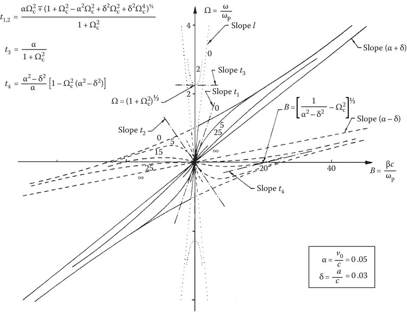
FIGURE 10C.1
The ω−β diagram normalized to the plasma frequency, for guided waves in a warm uniaxial drifting electron plasma for the case of the drift velocity v₀ greater than the acoustic velocity a. The numbers on the curves are the values of Ω_c, and the mode cutoff frequency of the empty guide ω_c normalized to the plasma frequency. (Reprinted with permission from Kalluri, D., Waveguide modes of a warm drifting uniaxial electron plasma, *Proc. IEEE*, 58(2), 278–280, © February 1970 IEEE.)

Substituting Equation 10C.9 into Equation 10C.8, we obtain

(10C.10)

(Ω^{2} - B^{2}) [{(Ω - α B)}^{2} - δ^{2} B^{2} - 1] = Ω_{c}^{2} [{(Ω - α B)}^{2} - δ^{2} B^{2}] .

$(Ω^{2} - B^{2}) [{(Ω - α B)}^{2} - δ^{2} B^{2} - 1] = Ω_{c}^{2} [{(Ω - α B)}^{2} - δ^{2} B^{2}] .$

This is a fourth-degree polynomial equation in Ω, B. The radius vector to each point on the diagram is proportional to the phase velocity [v_ϕ = c(Ω/B)] and the slope of the tangent at each point is proportional to the group velocity (v_g = c dΩ/dB). The Ω−B diagram has a double point at the origin and the tangents at this point are given by

(10C.11)

t_{1, 2} = \frac{α Ω_{c}^{2} \mp \sqrt{1 + Ω_{c}^{2} - α^{2} Ω_{c}^{2} + δ^{2} Ω_{c}^{4}}}{1 + Ω_{c}^{2}} .

$t_{1, 2} = \frac{α Ω_{c}^{2} \mp \sqrt{1 + Ω_{c}^{2} - α^{2} Ω_{c}^{2} + δ^{2} Ω_{c}^{4}}}{1 + Ω_{c}^{2}} .$

The diagram cuts the Ω-axis at $Ω = \mp {(1 + Ω_{c}^{2})}^{1 / 2}$ $Ω = \mp {(1 + Ω_{c}^{2})}^{1 / 2}$ and the tangent to the curve at this point is given by

(10C.12)

t_{3} = \frac{α}{1 + Ω_{c}^{2}} .

$t_{3} = \frac{α}{1 + Ω_{c}^{2}} .$

It cuts the B-axis at $B = {\{[1 / (α^{2} - δ^{2})] - Ω_{c}^{2}\}}^{1 / 2}$ $B = {\{[1 / (α^{2} - δ^{2})] - Ω_{c}^{2}\}}^{1 / 2}$ and the tangent at this point is given by

(10C.13)

t_{4} = \frac{α^{2} - δ^{2}}{α} [1 - Ω_{c}^{2} (α^{2} - δ^{2})] .

$t_{4} = \frac{α^{2} - δ^{2}}{α} [1 - Ω_{c}^{2} (α^{2} - δ^{2})] .$

The general characteristics of the Ω−B diagram for a given Ω_c may be obtained by considering the two extreme cases of Ω_c = 0 (one-dimensional case) and Ω_c = ∞. In the former case, the fourth-degree curve degenerates into two straight lines Ω = ±B and the hyperbola (Ω − αB)² − δ²B² − 1 = 0. In the latter case (Ω_c = ∞), the curve degenerates into two straight lines Ω = (α ∓ δ)B. The branches of the fourth-degree curve for any other Ω_c will be boxed by the compartments formed by the branches of the curves for the two extreme cases. Figures 10C.1 and 10C.2 illustrate this point. In these diagrams, one may identify [2,6] the “fast wave” whose phase velocity v_ϕ₁ > c(α − δ), the “slow wave” with phase velocity v_ϕ₂ < c(α − δ), and the “waveguide wave.” In Figure 10C.1, the Ω−B diagram is shown for α = 0.05 and δ = 0.03, the parameter being Ω_c. For ω < ω_p, one of these curves (e.g., the dashed curve marked Ω_c = 5) shows the existence of the backward waves (with positive group velocity and negative phase velocity) as well as a stationary wave (v_g = 0). However, these disappear for Ω_c ≥ (α² − δ²)^−1/2 (see, e.g., the dashed curve marked Ω_c = 25 of Figure 10C.1). Figure 10C.2 shows the Ω−B diagram for α < δ (α = 0.03, δ = 0.05). In Figure 10C.3, the phase characteristics of the waveguide wave for α = 0.05, δ = 0.03, and Ω_c = 0.1 are exhibited in great detail. It can be seen from this diagram that while the low-frequency cutoff for the forward waves of the waveguide wave is given by ${(1 + Ω_{c}^{2})}^{1 / 2}$ ${(1 + Ω_{c}^{2})}^{1 / 2}$ (point P, Figure 10C.3), there exist backward waves for a small band of frequencies (branch AP) below the cutoff frequency ${(1 + Ω_{c}^{2})}^{1 / 2}$ ${(1 + Ω_{c}^{2})}^{1 / 2}$ . This band extends in width as Ω_c decreases with a maximum value of α/(l + α). The transition of the waveguide wave from the forward wave type to the backward wave type takes place at a group velocity v_g = ct₃.

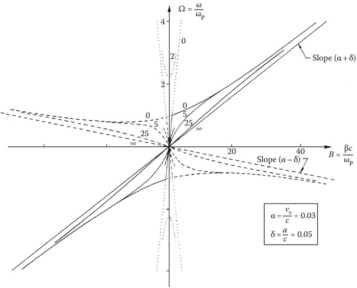
FIGURE 10C.2
The ω−β diagram normalized to the plasma frequency ω_p, for guided waves in a warm uniaxial drifting electron plasma for the case of the drift velocity v₀ less than the acoustic velocity a. The numbers on the curves are as given in Figure 10C.1. (Reprinted with permission from Kalluri, D., Waveguide modes of a warm drifting uniaxial electron plasma, *Proc. IEEE*, 58(2), 278–280, © February 1970 IEEE.)

FIGURE 10C.3
Phase characteristics of the “waveguide wave” of a warm uniaxial drifting electron plasma near the point Ω = [1 + (ω_c/ω_p)²]^1/2, where ω_c is the mode cutoff frequency of the empty guide. (Reprinted with permission from Kalluri, D., Waveguide modes of a warm drifting uniaxial electron plasma, *Proc. IEEE*, 58(2), 278–280, © February 1970 IEEE [7].)

References

1.Allis, W. P., Buchbaum, S. J., and Bers, A., Waves in Anisotropic Plasmas, MIT Press, Cambridge, MA, 1963.
2.Trivelpiece, A. W., Slow-Wave Propagation in Plasma Waveguides, San Francisco Press, San Francisco, CA, 1967.
3.Tuan, H. S., Mode theory of waveguide filled with warm uniaxial plasma, IEEE Trans. Microw. Theory Tech., MTT-17, 134–137, 1969.
4.Smullin, L. D. and Chorney, P., Propagation in ion loaded waveguide, Proceedings of the Symposium on Electronic Waveguides, Polytechnic Press, Brooklyn, NY, 1958.
5.Briggs, R. J., Electron–Stream Interaction with Plasmas, MIT Press, Cambridge, MA, 1964.
6.Articolo, G. A., Derivation of an equivalent dielectric tensor for a warm, drifting, lossy, electron plasma, J. Appl. Phys., 40, 1896–1902, 1969.
7.Kalluri, D., Waveguide modes of a warm drifting uniaxial electron plasma, Proc. IEEE, 58(2), 278–280, February 1970.

..................Content has been hidden....................

You can't read the all page of ebook, please click here login for view all page.

Table of Contents for Appendix 10C: Waveguide Modes of a Warm Drifting Uniaxial Electron Plasma

Create new playlist

Sign In

Sign Up

10C.1Introduction

10C.2Basic Equations

References

Table of Contents for
Appendix 10C: Waveguide Modes of a Warm Drifting Uniaxial Electron Plasma