The linear regression model is used for explaining the relationship between a single dependent variable known as Y and one or more X's independent variables known as input, predictor, or independent variables. The following two equations explain a linear regression scenario:

Equation 1 shows the formulation of a simple linear regression equation and equation 2 shows the multiple linear equations where many independent variables can be included. The dependent variable must be a continuous variable and the independent variables can be continuous and categorical. We are going to explain the multiple linear regression analysis by taking the Cars93_1.csv dataset, where the dependent variable is the price of cars and all the other variables are explanatory variables. The regression analysis includes:

The primary objective of a regression model is to estimate the beta parameters and minimize the error term epsilon:

Let's look at the relationship between various variables using a correlation plot:

#Scatterplot showing all the variables in the dataset

library(car);attach(Cars93_1)

> #12-"Rear.seat.room",13-"Luggage.room" has NA values need to remove them

> m<-cor(Cars93_1[,-c(12,13)])

> corrplot(m, method = "ellipse")

The preceding figure shows the relationship between various variables. From each ellipse we can get to know how the relationship: is it positive or negative, and is it strongly associated, moderately associated, or weakly associated? The correlation plot helps in taking a decision on which variables to keep for further investigation and which ones to remove from further analysis. The dark brown colored ellipse indicates perfect negative correlation and the dark blue colored ellipse indicates the perfect positive correlation. The narrower the ellipse, the higher the degree of correlation.

Given the number of variables in the dataset, it is quite difficult to read the scatterplot. Hence the correlation between all the variables can be represented using a correlation graph, as follows:

Correlation coefficients represented in bold blue color show higher degree of positive correlation and the ones with red color show higher degree of negative correlation.

The assumptions of a linear regression are as follows:

While fitting a multiple linear regression model, it is important to take care of the preceding assumptions. Let's look at the summary statistics from the multiple linear regression analysis and interpret the assumptions:

> #multiple linear regression model
> fit<-lm(MPG.Overall~.,data=Cars93_1)
> #model summary

> summary(fit)
Call:
lm(formula = MPG.Overall ~ ., data = Cars93_1)
Residuals:
Min 1Q Median 3Q Max
-5.0320 -1.4162 -0.0538 1.2921 9.8889
Coefficients:
Estimate Std. Error t value Pr(>|t|)
(Intercept) 2.808773 16.112577 0.174 0.86213
Price -0.053419 0.061540 -0.868 0.38842
EngineSize 1.334181 1.321805 1.009 0.31638
Horsepower 0.005006 0.024953 0.201 0.84160
RPM 0.001108 0.001215 0.912 0.36489
Rev.per.mile 0.002806 0.001249 2.247 0.02790 *
Fuel.tank.capacity -0.639270 0.262526 -2.435 0.01752 *
Length -0.059862 0.065583 -0.913 0.36459
Wheelbase 0.330572 0.156614 2.111 0.03847 *
Width 0.233123 0.265710 0.877 0.38338
Turn.circle 0.026695 0.197214 0.135 0.89273
Rear.seat.room -0.031404 0.182166 -0.172 0.86364
Luggage.room 0.206758 0.188448 1.097 0.27644
Weight -0.008001 0.002849 -2.809 0.00648 **
---
Signif. codes: 0 '***' 0.001 '**' 0.01 '*' 0.05 '.' 0.1 ' ' 1
Residual standard error: 2.835 on 68 degrees of freedom
(11 observations deleted due to missingness)
Multiple R-squared: 0.7533, Adjusted R-squared: 0.7062
F-statistic: 15.98 on 13 and 68 DF, p-value: 7.201e-16

In the previous multiple linear regression model using all the independent variables, we are predicting the mileage per gallon MPG.Overall variable. From the model summary, it is observed that few independent variables are statistically significant at 95% confidence level. The coefficient of determination R² which is known as the goodness of fit of a regression model is 75.33%. This implies that 75.33% variation in the dependent variable is explained by all the independent variables together. The formula for computing multiple R² is given next:

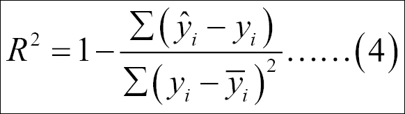
The preceding equation 4 calculated the coefficient of determination or percentage of variance explained by the regression model. The base line score to qualify for a good regression model is at least 80% as R square value; any R square value more than 80% is considered to be very good regression model. Since the R² is now less than 80%, we need to perform a few diagnostic tests on the regression results.

The estimated beta coefficients of the model:

> #estimated coefficients
> fit$coefficients
(Intercept) Price EngineSize Horsepower
2.808772930 -0.053419142 1.334180881 0.005005690
RPM Rev.per.mile Fuel.tank.capacity Length
0.001107897 0.002806093 -0.639270186 -0.059861997
Wheelbase Width Turn.circle Rear.seat.room
0.330572119 0.233123382 0.026694571 -0.031404262
Luggage.room Weight
0.206757968 -0.008001444
#residual values
fit$residuals
#fitted values from the model
fit$fitted.values
#what happened to NA
fit$na.action
> #ANOVA table from the model
> summary.aov(fit)
Df Sum Sq Mean Sq F value Pr(>F)
Price 1 885.7 885.7 110.224 7.20e-16 ***
EngineSize 1 369.3 369.3 45.959 3.54e-09 ***
Horsepower 1 37.4 37.4 4.656 0.03449 *
RPM 1 38.8 38.8 4.827 0.03143 *
Rev.per.mile 1 71.3 71.3 8.877 0.00400 **
Fuel.tank.capacity 1 147.0 147.0 18.295 6.05e-05 ***
Length 1 1.6 1.6 0.203 0.65392
Wheelbase 1 35.0 35.0 4.354 0.04066 *
Width 1 9.1 9.1 1.139 0.28969
Turn.circle 1 0.5 0.5 0.060 0.80774
Rear.seat.room 1 0.6 0.6 0.071 0.79032
Luggage.room 1 9.1 9.1 1.129 0.29170
Weight 1 63.4 63.4 7.890 0.00648 **
Residuals 68 546.4 8.0
---
Signif. codes: 0 '***' 0.001 '**' 0.01 '*' 0.05 '.' 0.1 ' ' 1
11 observations deleted due to missingness

From the preceding analysis of variance (ANOVA) table, it is observed that the variables Length, Width, turn circle, rear seat room, and luggage room are not statistically significant at 5% level of alpha. ANOVA shows the source of variation in dependent variable from any independent variable. It is important to apply ANOVA after the regression model to know which independent variable has significant contribution to the dependent variable:

> #visualizing the model statistics

> par(mfrow=c(1,2))

> plot(fit, col="dodgerblue4")

The residual versus fitted plot shows the randomness in residual values as we move along the fitted line. If the residual values display any pattern against the fitted values, the error term is not probably normal. The residual versus fitted graph indicates that there is no pattern that exists among the residual terms; the residuals are approximately normally distributed. Residual is basically that part of the model which cannot be explained by the model. There are few influential data points, for example, 42^nd, 39^th, and 83^rd as it is shown on the preceding graph, the normal quantile-quantile plot indicates except few influential data points all other standardized residual points follow a normal distribution. The straight line is the zero residual line and the red line is the pattern of residual versus fitted relationship. The scale versus location graph and the residuals versus leverage graph also validate the same observation that the residual term has no trend. The scale versus location plot takes the square root of the standardized residuals and plots it against the fitted values:

The confidence interval of the model coefficients at 95% confidence level can be calculated using the following code and also the prediction interval at 95% confidence level for all the fitted values can be calculated using the code below. The formula to compute the confidence interval is the model coefficient +/- standard error of model coefficient * 1.96:

> confint(fit,level=0.95)

2.5 % 97.5 %

(Intercept) -2.934337e+01 34.960919557

Price -1.762194e-01 0.069381145

EngineSize -1.303440e+00 3.971801771

Horsepower -4.478638e-02 0.054797758

RPM -1.315704e-03 0.003531499

Rev.per.mile 3.139667e-04 0.005298219

Fuel.tank.capacity -1.163133e+00 -0.115407347

Length -1.907309e-01 0.071006918

Wheelbase 1.805364e-02 0.643090600

Width -2.970928e-01 0.763339610

Turn.circle -3.668396e-01 0.420228772

Rear.seat.room -3.949108e-01 0.332102243

Luggage.room -1.692837e-01 0.582799642

Weight -1.368565e-02 -0.002317240

> head(predict(fit,interval="predict"))

fit lwr upr

1 31.47382 25.50148 37.44615

2 24.99014 18.80499 31.17528

3 22.09920 16.09776 28.10064

4 21.19989 14.95606 27.44371

5 21.62425 15.37929 27.86920

6 27.89137 21.99947 33.78328

The existence of influential data points or outlier values may deviate the model result, hence identification and curation of outlier data points in the regression model is very important:

# Deletion Diagnostics

influence.measures(fit)

The function belongs to the stats library, which computes some of the regression diagnostics for linear and generalized models. Any observation labeled with a star (*) implies an influential data point, that can be removed to make the model good:

# Index Plots of the influence measures

influenceIndexPlot(fit, id.n=3)

The influential data points are highlighted by their position in the dataset. In order to understand more about these influential data points, we can write the following command. The size of the red circle based on the cook's distance value indicates the order of influence. Cook's distance is a statistical method to identify data points which have more influence than other data points.

Generally, these are data points that are distant from other points in the data, either for the dependent variable or one or more independent variables:

> # A user friendly representation of the above

> influencePlot(fit,id.n=3, col="red")

StudRes Hat CookD

28 1.9902054 0.5308467 0.55386748

39 3.9711522 0.2193583 0.50994280

42 4.1792327 0.1344866 0.39504695

59 0.1676009 0.4481441 0.04065691

60 -2.1358078 0.2730012 0.34097909

77 -0.6448891 0.3980043 0.14074778

If we remove these influential data points from our model, we can see some improvement in the model goodness of fit and overall error for the model can be reduced. Removing all the influential points at one go is not a good idea; hence we will take a step-by-step approach to deleting these influential data points from the model and monitor the improvement in the model statistics:

> ## Regression after deleting the 28th observation

> fit.1<-lm(MPG.Overall~., data=Cars93_1[-28,])

> summary(fit.1)

Call:

lm(formula = MPG.Overall ~ ., data = Cars93_1[-28, ])

Residuals:

Min 1Q Median 3Q Max

-5.0996 -1.7005 0.4617 1.4478 9.4168

Coefficients:

Estimate Std. Error t value Pr(>|t|)

(Intercept) -6.314222 16.425437 -0.384 0.70189

Price -0.014859 0.063281 -0.235 0.81507

EngineSize 2.395780 1.399569 1.712 0.09156 .

Horsepower -0.022454 0.028054 -0.800 0.42632

RPM 0.001944 0.001261 1.542 0.12789

Rev.per.mile 0.002829 0.001223 2.314 0.02377 *

Fuel.tank.capacity -0.640970 0.256992 -2.494 0.01510 *

Length -0.065310 0.064259 -1.016 0.31311

Wheelbase 0.407332 0.158089 2.577 0.01219 *

Width 0.204212 0.260513 0.784 0.43587

Turn.circle 0.071081 0.194340 0.366 0.71570

Rear.seat.room -0.004821 0.178824 -0.027 0.97857

Luggage.room 0.156403 0.186201 0.840 0.40391

Weight -0.008597 0.002804 -3.065 0.00313 **

---

Signif. codes: 0 '***' 0.001 '**' 0.01 '*' 0.05 '.' 0.1 ' ' 1

Residual standard error: 2.775 on 67 degrees of freedom

(11 observations deleted due to missingness)

Multiple R-squared: 0.7638, Adjusted R-squared: 0.718

F-statistic: 16.67 on 13 and 67 DF, p-value: 3.39e-16

Regression output after deleting the most influential data point provides a significant improvement in the R2 value from 75.33% to 76.38%. Let's repeat the same activity and see the model's results:

> ## Regression after deleting the 28,39,42,59,60,77 observations

> fit.2<-lm(MPG.Overall~., data=Cars93_1[-c(28,42,39,59,60,77),])

> summary(fit.2)

Call:

lm(formula = MPG.Overall ~ ., data = Cars93_1[-c(28, 42, 39,

59, 60, 77), ])

Residuals:

Min 1Q Median 3Q Max

-3.8184 -1.3169 0.0085 0.9407 6.3384

Coefficients:

Estimate Std. Error t value Pr(>|t|)

(Intercept) 21.4720002 13.3375954 1.610 0.11250

Price -0.0459532 0.0589715 -0.779 0.43880

EngineSize 2.4634476 1.0830666 2.275 0.02641 *

Horsepower -0.0313871 0.0219552 -1.430 0.15785

RPM 0.0022055 0.0009752 2.262 0.02724 *

Rev.per.mile 0.0016982 0.0009640 1.762 0.08307 .

Fuel.tank.capacity -0.6566896 0.1978878 -3.318 0.00152 **

Length -0.0097944 0.0613705 -0.160 0.87372

Wheelbase 0.2298491 0.1288280 1.784 0.07929 .

Width -0.0877751 0.2081909 -0.422 0.67477

Turn.circle 0.0347603 0.1513314 0.230 0.81908

Rear.seat.room -0.2869723 0.1466918 -1.956 0.05494 .

Luggage.room 0.1828483 0.1427936 1.281 0.20514

Weight -0.0044714 0.0021914 -2.040 0.04557 *

---

Signif. codes: 0 '***' 0.001 '**' 0.01 '*' 0.05 '.' 0.1 ' ' 1

Residual standard error: 2.073 on 62 degrees of freedom

(11 observations deleted due to missingness)

Multiple R-squared: 0.8065, Adjusted R-squared: 0.7659

F-statistic: 19.88 on 13 and 62 DF, p-value: < 2.2e-16

Looking at the preceding output, we can conclude that the removal of outliers or influential data points adds robustness to the R-square value. Now we can conclude that 80.65% of the variation in the dependent variable is being explained by all the independent variables in the model.

Now, using studentised residuals against t-quantiles in a Q-Q plot, we can identify some more outliers data points, if any, to boost the model accuracy:

> # QQ plots of studentized residuals, helps identify outliers

> qqPlot(fit.2, id.n=5)

91 32 55 5 83

1 2 74 75 76

From the preceding Q-Q plot, it seems that the data is fairly normally distributed, except few outlier values such as 83^rd, 91^st, 32^nd, 55^th, and 5^th data points:

> ## Diagnostic Plots ###

> influenceIndexPlot(fit.2, id.n=3)

> influencePlot(fit.2, id.n=3, col="blue")

StudRes Hat CookD

5 2.1986298 0.2258133 0.30797166

8 -0.1448259 0.4156467 0.03290507

10 -0.7655338 0.3434515 0.14847534

83 3.7650470 0.2005160 0.45764995

91 -2.3672942 0.3497672 0.44770173

The problem of multicollinearity, that is, the correlation between predictor variables, needs to be verified for the final regression model. Variance Inflation Factor (VIF) is the measure typically used to estimate the multicollinearity. The formula to compute the VIF is 1/ (1-R² ). Any independent variable having a VIF value of more than 10 indicates multicollinearity; hence such variables need to be removed from the model. Deleting one variable at a time and then again checking the VIF for the model is the best way to do this:

> ### Variance Inflation Factors

> vif(fit.2)

Price EngineSize Horsepower RPM

4.799678 20.450596 18.872498 5.788160

Rev.per.mile Fuel.tank.capacity Length Wheelbase

3.736889 5.805824 15.200301 11.850645

Width Turn.circle Rear.seat.room Luggage.room

10.243223 4.006895 2.566413 2.935853

Weight

24.977015

Variable weight has the maximum VIF, hence deleting the variable make sense. After removing the variable, let's rerun the model and calculate the VIF:

## Regression after deleting the weight variable

fit.3<-lm(MPG.Overall~ Price+EngineSize+Horsepower+RPM+Rev.per.mile+

Fuel.tank.capacity+Length+Wheelbase+Width+Turn.circle+

Rear.seat.room+Luggage.room, data=Cars93_1[-c(28,42,39,59,60,77),])

summary(fit.3)

> vif(fit.3)

Price EngineSize Horsepower RPM

4.575792 20.337181 15.962349 5.372388

Rev.per.mile Fuel.tank.capacity Length Wheelbase

3.514992 4.863944 14.574352 11.013850

Width Turn.circle Rear.seat.room Luggage.room

10.240036 3.965132 2.561947 2.935690

## Regression after deleting the Enginesize variable

fit.4<-lm(MPG.Overall~ Price+Horsepower+RPM+Rev.per.mile+

Fuel.tank.capacity+Length+Wheelbase+Width+Turn.circle+

Rear.seat.room+Luggage.room, data=Cars93_1[-c(28,42,39,59,60,77),])

summary(fit.4)

vif(fit.4)

## Regression after deleting the Length variable

fit.5<-lm(MPG.Overall~ Price+Horsepower+RPM+Rev.per.mile+

Fuel.tank.capacity+Wheelbase+Width+Turn.circle+

Rear.seat.room+Luggage.room, data=Cars93_1[-c(28,42,39,59,60,77),])

summary(fit.5)

> vif(fit.5)

Price Horsepower RPM Rev.per.mile

4.419799 8.099750 2.595250 3.232048

Fuel.tank.capacity Wheelbase Width Turn.circle

4.679088 8.231261 7.953452 3.357780

Rear.seat.room Luggage.room

2.393630 2.894959

The coefficients from the final regression model:

> coefficients(fit.5)

(Intercept) Price Horsepower RPM

29.029107454 -0.089498236 -0.014248077 0.001071072

Rev.per.mile Fuel.tank.capacity Wheelbase Width

0.001591582 -0.769447316 0.130876817 -0.047053999

Turn.circle Rear.seat.room Luggage.room

-0.072030390 -0.240332275 0.216155256

Now we can conclude that there is no multicollinearity in the preceding regression model. We can write the final multiple linear regression equation as follows:

The estimated model parameters can be interpreted as, for one unit change in the price variable, the MPG overall is predicted to change by 0.09 unit. Likewise, the estimated model coefficients can be interpreted for all the other independent variables. If we know the values of these independent variables, we can predict the likely value of the dependent variable MPG overall by using the previous equation.