
We are going to apply dimensionality reduction procedure, both model-based approach and principal component-based approach, on the dataset to come up with less number of features so that we can use those features for classification of the customers into defaulters and no-defaulters.
For practical project, we have considered a dataset default of credit card clients.csv, which contains 30,000 samples and 24 attributes or dimensions. We are going to apply two different methods of feature reduction: the traditional way and the modern machine learning way.
The following are descriptions for the attributes from the dataset:
X1: Amount of the given credit (NT dollar). It includes both the individual consumer credit and his/her family (supplementary) credit.X2: Gender (1 = male; 2 = female).X3: Education (1 = graduate school; 2 = university; 3 = high school; 4 = others).X4: Marital status (1 = married; 2 = single; 3 = others).X5: Age (year).X6 - X11: History of past payment. We tracked the past monthly payment records (from April to September, 2005) as follows:X6= the repayment status in September, 2005X7 = the repayment status in August, 2005; . . .X11 = the repayment status in April, 2005. The measurement scale for the repayment status is: -1 = pay duly; 1 = payment delay for one month; 2 = payment delay for two months; . . . 8 = payment delay for eight months; 9 = payment delay for nine months, and so on.
X12-X17: Amount of bill statement (NT dollar).X12 = amount of bill statement in September, 2005;X13 = amount of bill statement in August, 2005; . . .X17 = amount of bill statement in April, 2005.
X18-X23: Amount of previous payment (NT dollar).X18 = amount paid in September, 2005;X19 = amount paid in August, 2005; . . .X23 = amount paid in April, 2005.
Let's get the dataset and do the necessary normalization and transformation:
> setwd("select the working directory")

> default<-read.csv("default.csv")

corrplot::corrplot(cor(df),method="ellipse")
From the preceding correlations matrix, it is clear that there are some strong correlations between different variables from X12 to X17, which possibly can be clubbed together as linear combinations using PCA. The following graph shows the correlations between different variables:
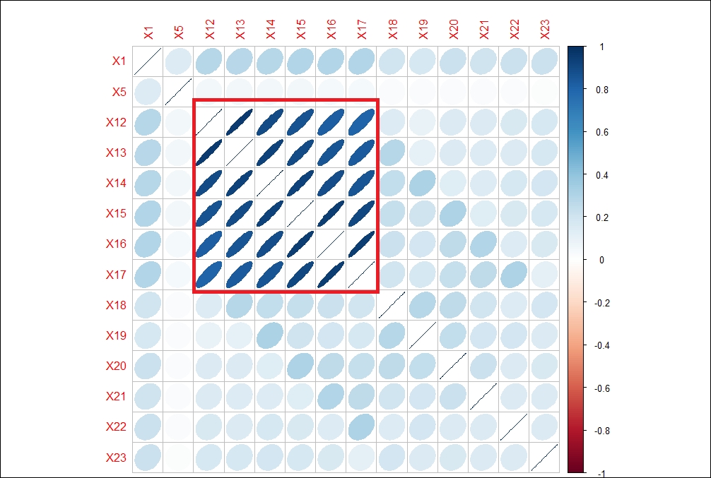
In the previous correlations graph, the strength of the correlation is reflected by the size of the ellipse and the color varying from red to blue. The blue ellipses indicate positive correlation and the white ones show no correlation. Variable X12 has a high degree of positive correlation with variables X13 to X17, with a correlation value of more than 80%.
Row number 1 contains the variable description and there are some columns which are categorical; we need to remove those from our dataset. Some other variables are shown as categorical and hence need to be converted back to numeric mode:
> df<-default[-1,-c(1,3:5,7:12,25)]

> func1<-function(x){

+ as.numeric(x)

+ }

> df<-as.data.frame(apply(df,2,func1))

> normalize-function(x){

+ (x-mean(x))

+ }
Using func1, we convert the non-numeric variables into numeric so that we can apply the normalization function (normalize), which is doing data normalization. After applying normalization, the dataset will look like the one as shown next. To apply principal component analysis, either we can use mean normalized dataset as an input or we can use the base dataset with correlations or a covariance matrix as an input. If we are not going to normalize the dataset, the variable with the highest variance will become the first principal component and hence will dominate other relevant principal components:
> dn<-as.data.frame(apply(df,2,normalize))

> str(dn)

'data.frame': 30000 obs. of 14 variables:

$ X1 : num -147484 -47484 -77484 -117484 -117484 ...

$ X5 : num -11.49 -9.49 -1.49 1.51 21.51 ...

$ X12: num -47310 -48541 -21984 -4233 -42606 ...

$ X13: num -46077 -47454 -35152 -946 -43509 ...

$ X14: num -46324 -44331 -33454 2278 -11178 ...

$ X15: num -43263 -39991 -28932 -14949 -22323 ...

$ X16: num -40311 -36856 -25363 -11352 -21165 ...

$ X17: num -38872 -35611 -23323 -9325 -19741 ...

$ X18: num -5664 -5664 -4146 -3664 -3664 ...

$ X19: num -5232 -4921 -4421 -3902 30760 ...

$ X20: num -5226 -4226 -4226 -4026 4774 ...

$ X21: num -4826 -3826 -3826 -3726 4174 ...

$ X22: num -4799 -4799 -3799 -3730 -4110 ...

$ X23: num -5216 -3216 -216 -4216 -4537 ...
Running principal component analysis:
> options(digits = 2)

> pca1<-princomp(df,scores = T, cor = T)

> summary(pca1)

Importance of components:

Comp.1 Comp.2 Comp.3 Comp.4 Comp.5 Comp.6 Comp.7 Comp.8 Comp.9 Comp.10 Comp.11

Standard deviation 2.43 1.31 1.022 0.962 0.940 0.934 0.883 0.852 0.841 0.514 0.2665

Proportion of Variance 0.42 0.12 0.075 0.066 0.063 0.062 0.056 0.052 0.051 0.019 0.0051

Cumulative Proportion 0.42 0.55 0.620 0.686 0.749 0.812 0.867 0.919 0.970 0.989 0.9936

Comp.12 Comp.13 Comp.14

Standard deviation 0.2026 0.1592 0.1525

Proportion of Variance 0.0029 0.0018 0.0017

Cumulative Proportion 0.9965 0.9983 1.0000
Principal component (PC) 1 explains 42% variation in the dataset and principal component 2 explains 12% variation in the dataset. This means that first PC has closeness to 42% of the total data points in the n-dimensional space. From the preceding results, it is clear that the first 8 principal components capture 91.9% variation in the dataset. Rest 8% variation in the dataset is explained by 6 other principal components. Now the question is how many principal components should be chosen. The general rule of thumb is 80-20, if 80% variation in the data can be explained by 20% of the principal components. There are 14 variables; we have to look at how many components explain 80% variation in the dataset cumulatively. Hence, it is recommended, based on the 80:20 Pareto principle, taking 6 principal components which explain 81% variation cumulatively.
In a multivariate dataset, the correlation between the component and the original variables is called the component loading. The loadings of the principal components are as follows:
> #Loadings of Principal Components

> pca1$loadings

Loadings:

Comp.1 Comp.2 Comp.3 Comp.4 Comp.5 Comp.6 Comp.7 Comp.8 Comp.9 Comp.10 Comp.11 Comp.12 Comp.13 Comp.14

X1 -0.165 0.301 0.379 0.200 0.111 0.822

X5 0.870 -0.338 -0.331

X12 -0.372 -0.191 0.567 0.416 0.433 0.184 -0.316

X13 -0.383 -0.175 0.136 0.387 -0.345 -0.330 0.645

X14 -0.388 -0.127 -0.114 -0.121 0.123 -0.485 -0.496 -0.528

X15 -0.392 -0.120 0.126 -0.205 -0.523 0.490 0.362 0.346

X16 -0.388 -0.106 0.107 -0.420 0.250 -0.718 -0.227

X17 -0.381 0.165 -0.489 0.513 -0.339 0.428

X18 -0.135 0.383 -0.173 -0.362 -0.226 -0.201 0.749

X19 -0.117 0.408 -0.201 -0.346 -0.150 0.407 -0.280 -0.578 0.110 0.147 0.125

X20 -0.128 0.392 -0.122 -0.245 0.239 -0.108 0.785 -0.153 0.145 -0.125

X21 -0.117 0.349 0.579 -0.499 -0.462 0.124 -0.116

X22 -0.114 0.304 0.609 0.193 0.604 0.164 -0.253

X23 -0.106 0.323 0.367 -0.658 -0.411 -0.181 -0.316

Comp.1 Comp.2 Comp.3 Comp.4 Comp.5 Comp.6 Comp.7 Comp.8 Comp.9 Comp.10 Comp.11 Comp.12 Comp.13 Comp.14

SS loadings 1.000 1.000 1.000 1.000 1.000 1.000 1.000 1.000 1.000 1.000 1.000 1.000 1.000 1.000

Proportion Var 0.071 0.071 0.071 0.071 0.071 0.071 0.071 0.071 0.071 0.071 0.071 0.071 0.071 0.071

Cumulative Var 0.071 0.143 0.214 0.286 0.357 0.429 0.500 0.571 0.643 0.714 0.786 0.857 0.929 1.000

> pca1

Call:

princomp(x = df, cor = T, scores = T)

Standard deviations:

Comp.1 Comp.2 Comp.3 Comp.4 Comp.5 Comp.6 Comp.7 Comp.8 Comp.9 Comp.10

2.43 1.31 1.02 0.96 0.94 0.93 0.88 0.85 0.84 0.51

Comp.11 Comp.12 Comp.13 Comp.14

0.27 0.20 0.16 0.15

14 variables and 30000 observations.
The following graph indicates the percentage variance explained by the principal components:
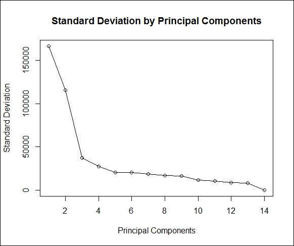
Following scree plot shows how many principal components we should retain for the dataset:
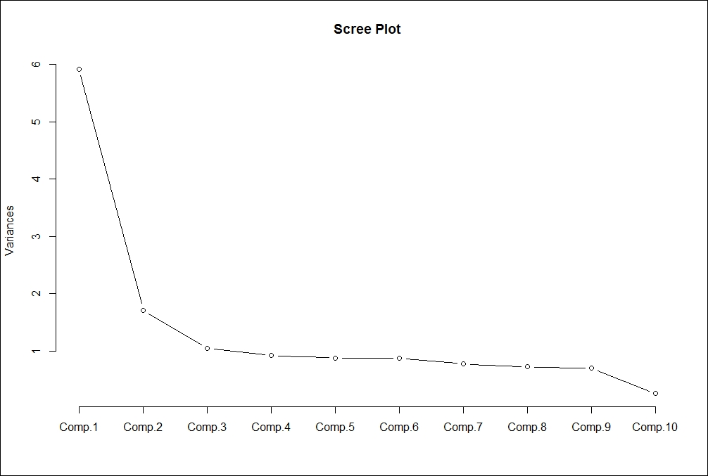
From the preceding scree plot, it is concluded that the first principal component has the highest variance, then second and third respectively. From the graph, three principal components have higher variance than the other principal components.
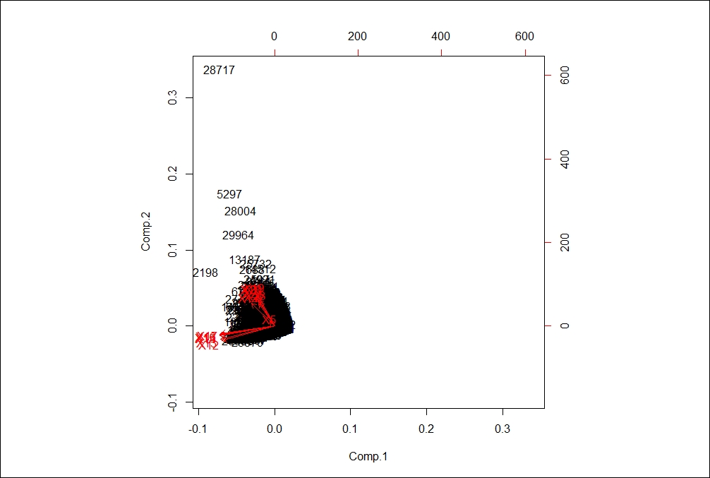
Following biplot indicates the existence of principal components in a n-dimensional space:
The diagonal elements of the covariance matrix are the variances of the variables; the off-diagonal variables are covariance between different variables:
> diag(cov(df))

X1 X5 X12 X13 X14 X15 X16 X17 X18 X19 X20

1.7e+10 8.5e+01 5.4e+09 5.1e+09 4.8e+09 4.1e+09 3.7e+09 3.5e+09 2.7e+08 5.3e+08 3.1e+08

X21 X22 X23

2.5e+08 2.3e+08 3.2e+08
The interpretation of scores is little bit tricky because they do not have any meaning until and unless you use them to plot on a straight line as defined by the eigen vector. PC scores are the co-ordinates of each point with respect to the principal axis. Using eigen values you can extract eigen vectors which describe a straight line to explain the PCs. The PCA is a form of multidimensional scaling as it represents data in a lower dimension without losing much information about the variables. The component scores are basically the linear combination of loading times the mean centred scaled dataset.
When we deal with multivariate data, it is really difficult to visualize and build models around it. In order to reduce the features, PCA is used; it reduces the dimensions so that we can plot, visualize, and predict the future, in a lower dimension. The principal components are orthogonal to each other, which means that they are uncorrelated. At the data pre-processing stage, the scaling function decides what type of input data matrix is required. If the mean centring approach is used as transformation then covariance matrix should be used as input data for PCA. If a scaling function does a standard z-score transformation, assuming standard deviation is equal to 1, then correlation matrix should be used as input data.
Now the question is where to apply which transformation. If the variables are highly skewed then z-score transformation and PCA based on correlation should be used. If the input data is approximately symmetric then mean centring approach and PCA based on covariance should be applied.
Now, let's look at the principal component scores:
> #scores of the components

> pca1$scores[1:10,]

Comp.1 Comp.2 Comp.3 Comp.4 Comp.5 Comp.6 Comp.7 Comp.8 Comp.9 Comp.10 Comp.11 Comp.12 Comp.13 Comp.14

[1,] 1.96 -0.54 -1.330 0.1758 -0.0175 0.0029 0.013 -0.057 -0.22 0.020 0.0169 0.0032 -0.0082 0.00985

[2,] 1.74 -0.22 -0.864 0.2806 -0.0486 -0.1177 0.099 -0.075 0.29 -0.073 -0.0055 -0.0122 0.0040 0.00072

[3,] 1.22 -0.28 -0.213 0.0082 -0.1269 -0.0627 -0.014 -0.084 -0.28 -0.016 0.1125 0.0805 0.0413 -0.05711

[4,] 0.54 -0.67 -0.097 -0.2924 -0.0097 0.1086 -0.134 -0.063 -0.60 0.144 0.0017 -0.1381 -0.0183 -0.05794

[5,] 0.85 0.74 1.392 -1.6589 0.3178 0.5846 -0.543 -1.113 -1.24 -0.038 -0.0195 -0.0560 0.0370 -0.01208

[6,] 0.54 -0.71 -0.081 -0.2880 -0.0924 0.1145 -0.194 -0.015 -0.58 0.505 0.0276 -0.1848 -0.0114 -0.14273

[7,] -15.88 -0.96 -1.371 -1.1334 0.3062 0.0641 0.514 0.771 0.99 -2.890 -0.4219 0.4631 0.3738 0.32748

[8,] 1.80 -0.29 -1.182 0.4394 -0.0620 -0.0440 0.076 -0.013 0.26 0.046 0.0484 0.0584 0.0268 -0.04504

[9,] 1.41 -0.21 -0.648 0.1902 -0.0653 -0.0658 0.040 0.122 0.33 -0.028 -0.0818 0.0296 -0.0605 0.00106

[10,] 1.69 -0.18 -0.347 -0.0891 0.5969 -0.2973 -0.453 -0.140 -0.74 -0.137 0.0248 -0.0218 0.0028 0.00423
Larger eigen values indicate larger variation in a dimension. The following script shows how to compute eigen values and eigen vectors from the correlation matrix:
> eigen(cor(df),TRUE)$values

[1] 5.919 1.716 1.045 0.925 0.884 0.873 0.780 0.727 0.707 0.264 0.071 0.041 0.025 0.023

head(eigen(cor(df),TRUE)$vectors)

[,1] [,2] [,3] [,4] [,5] [,6] [,7] [,8] [,9] [,10] [,11] [,12] [,13]

[1,] -0.165 0.301 0.379 0.2004 -0.035 -0.078 0.1114 0.0457 0.822 -0.0291 -0.00617 -0.0157 0.00048

[2,] -0.033 0.072 0.870 -0.3385 0.039 0.071 -0.0788 -0.0276 -0.331 -0.0091 0.00012 0.0013 -0.00015

[3,] -0.372 -0.191 0.034 0.0640 -0.041 -0.044 0.0081 -0.0094 -0.010 0.5667 0.41602 0.4331 0.18368

[4,] -0.383 -0.175 0.002 -0.0075 -0.083 -0.029 -0.0323 0.1357 -0.017 0.3868 0.03836 -0.3452 -0.32953

[5,] -0.388 -0.127 -0.035 -0.0606 -0.114 0.099 -0.1213 -0.0929 0.019 0.1228 -0.48469 -0.4957 0.08662

[6,] -0.392 -0.120 -0.034 -0.0748 -0.029 0.014 0.1264 -0.0392 -0.019 -0.2052 -0.52323 0.4896 0.36210

[,14]

[1,] 0.0033

[2,] 0.0011

[3,] -0.3164

[4,] 0.6452

[5,] -0.5277

[6,] 0.3462
The standard deviation of the individual principal components and the mean of all the principal components is as follows:
> pca1$sdev

Comp.1 Comp.2 Comp.3 Comp.4 Comp.5 Comp.6 Comp.7 Comp.8 Comp.9 Comp.10 Comp.11 Comp.12 Comp.13 Comp.14

2.43 1.31 1.02 0.96 0.94 0.93 0.88 0.85 0.84 0.51 0.27 0.20 0.16 0.15

> pca1$center

X1 X5 X12 X13 X14 X15 X16 X17 X18 X19 X20 X21 X22 X23

-9.1e-12 -1.8e-15 -6.8e-13 -3.0e-12 4.2e-12 4.1e-12 -1.4e-12 5.1e-13 7.0e-14 4.4e-13 2.9e-13 2.7e-13 -2.8e-13 -3.9e-13
Using the normalized data, and with no correlations table as an input, the following result is obtained. There is no difference in the output as we got the pca2 model in comparison to pca1:
> pca2<-princomp(dn)

> summary(pca2)

Importance of components:

Comp.1 Comp.2 Comp.3 Comp.4 Comp.5 Comp.6 Comp.7 Comp.8 Comp.9 Comp.10 Comp.11 Comp.12 Comp.13 Comp.14

Standard deviation 1.7e+05 1.2e+05 3.7e+04 2.8e+04 2.1e+04 2.0e+04 1.9e+04 1.7e+04 1.6e+04 1.2e+04 1.0e+04 8.8e+03 8.2e+03 9.1e+00

Proportion of Variance 6.1e-01 3.0e-01 3.1e-02 1.7e-02 9.4e-03 9.0e-03 7.5e-03 6.4e-03 5.8e-03 3.0e-03 2.4e-03 1.7e-03 1.5e-03 1.8e-09

Cumulative Proportion 6.1e-01 9.1e-01 9.4e-01 9.5e-01 9.6e-01 9.7e-01 9.8e-01 9.9e-01 9.9e-01 9.9e-01 1.0e+00 1.0e+00 1.0e+00 1.0e+00
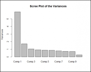
The next screen plot indicates that three principal components constitute most of the variation in the dataset. The x axis shows the principal components and the y axis shows the standard deviation (variance = square of the standard deviation).
The following script shows the plot being created:
> result<-round(summary(pca2)[1]$sdev,0)

> #scree plot

> plot(result, main = "Standard Deviation by Principal Components",

+ xlab="Principal Components",ylab="Standard Deviation",type='o')
Using the prcomp() function, which uses the SVD method to perform dimensionality reduction can be analysed as follows. prcomp() method accepts raw dataset as input and it has a built in argument which requires to make the scaling as true:
> pca<-prcomp(df,scale. = T)

> summary(pca)

Importance of components:

PC1 PC2 PC3 PC4 PC5 PC6 PC7 PC8 PC9 PC10

Standard deviation 2.433 1.310 1.0223 0.9617 0.9400 0.9342 0.8829 0.8524 0.8409 0.5142

Proportion of Variance 0.423 0.123 0.0746 0.0661 0.0631 0.0623 0.0557 0.0519 0.0505 0.0189

Cumulative Proportion 0.423 0.545 0.6200 0.6861 0.7492 0.8115 0.8672 0.9191 0.9696 0.9885

PC11 PC12 PC13 PC14

Standard deviation 0.26648 0.20263 0.15920 0.15245

Proportion of Variance 0.00507 0.00293 0.00181 0.00166

Cumulative Proportion 0.99360 0.99653 0.99834 1.00000
From the result we can see that there is little variation in the two methods. The SVD approach also shows that the first 8 components explain 91.91% variation in the dataset. From the documentation of prcomp and princomp, there is no difference in the type of PCA, but there is a difference in the method used to calculate PCA. The two methods are spectral decomposition and singular decomposition.
In spectral decomposition, as shown in the princomp function, the calculation is done using eigen on the correlation or covariance matrix. Using the prcomp method, the calculation is done by the SVD method.
To get the rotation matrix, which is equivalent to the loadings matrix in the princomp() method, we can use the following script:
> summary(pca)$rotation

PC1 PC2 PC3 PC4 PC5 PC6 PC7 PC8 PC9 PC10 PC11

X1 0.165 0.301 -0.379 0.2004 -0.035 0.078 -0.1114 -0.04567 0.822 -0.0291 0.00617

X5 0.033 0.072 -0.870 -0.3385 0.039 -0.071 0.0788 0.02765 -0.331 -0.0091 -0.00012

X12 0.372 -0.191 -0.034 0.0640 -0.041 0.044 -0.0081 0.00937 -0.010 0.5667 -0.41602

X13 0.383 -0.175 -0.002 -0.0075 -0.083 0.029 0.0323 -0.13573 -0.017 0.3868 -0.03836

X14 0.388 -0.127 0.035 -0.0606 -0.114 -0.099 0.1213 0.09293 0.019 0.1228 0.48469

X15 0.392 -0.120 0.034 -0.0748 -0.029 -0.014 -0.1264 0.03915 -0.019 -0.2052 0.52323

X16 0.388 -0.106 0.034 -0.0396 0.107 0.099 0.0076 0.04964 -0.024 -0.4200 -0.06824

X17 0.381 -0.094 0.018 0.0703 0.165 -0.070 -0.0079 -0.00015 -0.059 -0.4888 -0.51341

X18 0.135 0.383 0.173 -0.3618 -0.226 -0.040 0.2010 -0.74901 -0.020 -0.0566 -0.04763

X19 0.117 0.408 0.201 -0.3464 -0.150 -0.407 0.2796 0.57842 0.110 0.0508 -0.14725

X20 0.128 0.392 0.122 -0.2450 0.239 0.108 -0.7852 0.06884 -0.153 0.1449 -0.00015

X21 0.117 0.349 0.062 0.0946 0.579 0.499 0.4621 0.07712 -0.099 0.1241 0.11581

X22 0.114 0.304 -0.060 0.6088 0.193 -0.604 -0.0143 -0.16435 -0.253 0.0601 0.09944

X23 0.106 0.323 -0.050 0.3672 -0.658 0.411 -0.0253 0.18089 -0.316 -0.0992 -0.03495

PC12 PC13 PC14

X1 -0.0157 0.00048 -0.0033

X5 0.0013 -0.00015 -0.0011

X12 0.4331 0.18368 0.3164

X13 -0.3452 -0.32953 -0.6452

X14 -0.4957 0.08662 0.5277

X15 0.4896 0.36210 -0.3462

X16 0.2495 -0.71838 0.2267

X17 -0.3386 0.42770 -0.0723

X18 0.0693 0.04488 0.0846

X19 0.0688 -0.03897 -0.1249

X20 -0.1247 -0.02541 0.0631

X21 -0.0010 0.08073 -0.0423

X22 0.0694 -0.09520 0.0085

X23 -0.0277 0.01719 -0.0083
The rotated dataset can be retrieved by using argument x from the summary result of the prcomp() method:
> head(summary(pca)$x)

PC1 PC2 PC3 PC4 PC5 PC6 PC7 PC8 PC9 PC10 PC11 PC12

[1,] -1.96 -0.54 1.330 0.1758 -0.0175 -0.0029 -0.013 0.057 -0.22 0.020 -0.0169 0.0032

[2,] -1.74 -0.22 0.864 0.2806 -0.0486 0.1177 -0.099 0.075 0.29 -0.073 0.0055 -0.0122

[3,] -1.22 -0.28 0.213 0.0082 -0.1269 0.0627 0.014 0.084 -0.28 -0.016 -0.1125 0.0805

[4,] -0.54 -0.67 0.097 -0.2924 -0.0097 -0.1086 0.134 0.063 -0.60 0.144 -0.0017 -0.1381

[5,] -0.85 0.74 -1.392 -1.6588 0.3178 -0.5846 0.543 1.113 -1.24 -0.038 0.0195 -0.0560

[6,] -0.54 -0.71 0.081 -0.2880 -0.0924 -0.1145 0.194 0.015 -0.58 0.505 -0.0276 -0.1848

PC13 PC14

[1,] -0.0082 -0.00985

[2,] 0.0040 -0.00072

[3,] 0.0413 0.05711

[4,] -0.0183 0.05794

[5,] 0.0370 0.01208

[6,] -0.0114 0.14273

> biplot(prcomp(df,scale. = T))
The orthogonal red lines indicate the principal components that explain the entire dataset.
Having discussed various methods of variable reduction, what is going to be the output; the output should be a new dataset, in which all the principal components will be uncorrelated with each other. This dataset can be used for any task such as classification, regression, or clustering, among others. From the results of the principal component analysis how we get the new dataset; let's have a look at the following script:
> #calculating Eigen vectors

> eig<-eigen(cor(df))

> #Compute the new dataset

> eigvec<-t(eig$vectors) #transpose the eigen vectors

> df_scaled<-t(dn) #transpose the adjusted data

> df_new<-eigvec %*% df_scaled

> df_new<-t(df_new)

> colnames(df_new)<-c("PC1","PC2","PC3","PC4",

+ "PC5","PC6","PC7","PC8",

+ "PC9","PC10","PC11","PC12",

+ "PC13","PC14")

> head(df_new)

PC1 PC2 PC3 PC4 PC5 PC6 PC7 PC8 PC9 PC10 PC11 PC12

[1,] 128773 -19470 -49984 -27479 7224 10905 -14647 -4881 -113084 -2291 1655 2337

[2,] 108081 11293 -12670 -7308 3959 2002 -3016 -1662 -32002 -9819 -295 920

[3,] 80050 -7979 -24607 -11803 2385 3411 -6805 -3154 -59324 -1202 7596 7501

[4,] 37080 -39164 -41935 -23539 2095 9931 -15015 -4291 -92461 12488 -11 -7943

[5,] 77548 356 -50654 -38425 7801 20782 -19707 -28953 -88730 -12624 -9028 -4467

[6,] 34793 -42350 -40802 -22729 -2772 9948 -17731 -2654 -91543 37090 2685 -10960

PC13 PC14

[1,] -862 501

[2,] -238 -97

[3,] 2522 -4342

[4,] -1499 -4224

[5,] 3331 -9412

[6,] -1047 -10120