
In this chapter, we are going to discuss about various methods to reduce data dimensions in performing analysis. In data mining, traditionally people used to apply principal component analysis (PCA) as a method to reduce the dimensionality in data. Though now in the age of big data, PCA is still valid, however along with that, many other techniques are being used to reduce dimensions. With the growth of data in volumes and variety, the dimension of data has been continuously on the rise. Dimensionality reduction techniques have many applications in different industries, such as in image processing, speech recognition, recommendation engines, text processing, and so on. The main problem in these application areas is not only high dimensional data but also high sparsity. Sparsity means that many columns in the dataset will have missing or blank values.
In this chapter, we will implement dimensionality reduction techniques such as PCA, singular value decomposition (SVD), and iterative feature selection method using a practical data set and R programming language.
In this chapter, we are going to discuss:
- Why dimensionality reduction is a business problem and what impact it may have on the predictive models
- What are the different techniques, with their respective positives and negatives, and data requirements and more
- Which technique to apply and in what situations, with little bit of mathematics behind the calculation
- An R programming based implementation and interpretation of results in a project
In various statistical analysis models, especially showing a cause and impact relationship between dependent variable and a set of independent variables, if the number of independent variables increases beyond a manageable stage (for example, 100 plus), then it is quite difficult to interpret each and every variable. For example, in weather forecast, nowadays low cost sensors are being deployed at various places and those sensors provide signals and data are being stored in the database. When 1000 plus sensors provide data, it is important to understand the pattern or at least which all sensors are meaningful in performing the desired task.
Another example, from a business standpoint, is that if more than 30 features are impacting a dependent variable (for example, Sales), as a business owner I cannot regulate all 30 factors and cannot form strategies for 30 dimensions. Of course, as a business owner I would be interested in looking at 3-4 dimensions that should explain 80% of the dependent variable in the data. From the preceding two examples, it is pretty clear that dimensionality is still a valid business problem. Apart from business and volume, there are other reasons such as computational cost, storage cost of data, and more, if a set of dimensions are not at all meaningful for the target variable or target function why would I store it in my database.
Dimensionality reduction is useful in big data mining applications in performing both supervised learning and unsupervised learning-based tasks, to:
- Identify the pattern how the variables work together
- Display the relationship in a low dimensional space
- Compress the data for further analysis so that redundant features can be removed
- Avoid overfitting as reduced feature set with reduced degrees of freedom does that
- Running algorithms on a reduced feature set would be much more faster than the base features
Two important aspects of data dimensionality are, first, variables that are highly correlated indicate high redundancy in the data, and the second, most important dimensions always have high variance. While working on dimension reduction, it is important to take note of these aspects and make necessary amendments to the process.
Hence, it is important to reduce the dimensions. Also, it is not a good idea to focus on many variables to control or regulate the target variable in a predictive model. In a multivariate study, the correlation between various independent variables affect the empirical likelihood function and affects the eigen values and eigen vectors through covariance matrix.
The dimensionality reduction techniques can be classified into two major groups: parametric or model-based feature reduction and non-parametric feature reduction. In non-parametric feature reduction technique, the data dimension is reduced first and then the resulting data can be used to create any classification or predictive model, supervised or unsupervised. However, the parametric-based method emphasizes on monitoring the overall performance of a model and its accuracy by changing the features and hence deciding how many features are needed to represent the model. The following are the techniques generally used in data mining literature to reduce data dimensions:
- Non-parametric:
- PCA method
- Parametric method
- Forward feature selection
- Backward feature selection
We are going to discuss these methods in detail with the help of a dataset using R programming language. Apart from these techniques mentioned earlier, there are few more methods but not that popular, such as removing variables with low variance as they don't add much information to the target variable and also removing variables with many missing values. The latter comes under the missing value treatment method, but can still be used to reduce the features in a high dimensional dataset. There are two methods in R, prcomp() and princomp(), but they use two slightly different methods; princomp() uses eigen vectors and prcomp() uses SVD method. Some researchers favor prcomp() as a method over princomp() method. We are going to use two different methods here.
The usage of the technique actually depends upon the researcher; what he is looking at from the data. If you are looking at hidden features and want to represent the data in a low dimensional space, PCA is the method one should choose. If you are looking at building a good classification or prediction model, then it is not a good idea to perform PCA first; you should ideally include all the features and remove the redundant ones by any parametric method, such as forward or backward. Selection of techniques vary based on data availability, the problem statement, and the task that someone is planning to perform.
PCA is a multivariate statistical data analysis technique applicable for datasets with numeric variables only, which computes linear combinations of the original variables and those principal components are orthogonal to each other in the feature space. PCA is a method that uses eigen values and eigen vectors to compute the principal components, which is a linear combination of original variables. PCA can be used in regression modelling in order to remove the problem of multicollinearity in the dataset and can also be used in clustering exercise in order to understand unique group behaviors or segments existing in the dataset.
PCA assumes that the variables are linearly associated to form principal components and variables with high variance do not necessarily represent the best feature. The principal component analysis is based on a few theorems:
- The inverse of an orthogonal matrix is its transpose
- The original matrix times the transposed version of the original matrix are both symmetric
- A matrix is symmetric if it is an orthogonally diagonalizable matrix
- It uses variance matrix, not the correlation matrix to compute components
Following are the steps to perform principal component analysis:
- Get a numerical dataset. If you have any categorical variable, remove it from the dataset so that mathematical computation can happen on the remaining variables.
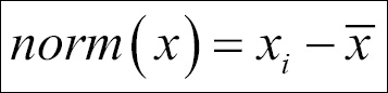
- In order to make the PCA work properly, data normalization should be done. This is done by deducting the mean of the column from each of the values for all the variables; ensure that the mean of the variables of the transformed data should be equal to 0.
We applied the following normalization formula:
- Calculate the covariance matrix on the reduced dataset. Covariance is a measure of two variables. A covariance matrix is a display of all the possible covariance values between all the different dimensions:
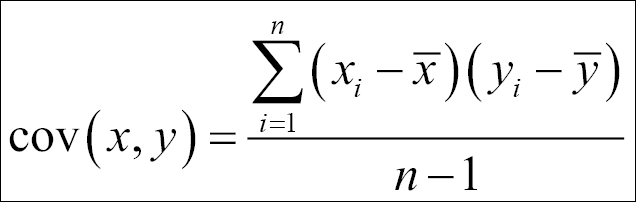
The sign of covariance is more important than its value; a positive covariance value indicates that both dimensions increase together and vice versa. Similarly, a negative value of covariance indicates that with an increase in one dimension, the other dimension decreases. If the covariance value is zero, it shows that the two dimensions are independent of each other and there is no relationship.
- Calculate the eigen vectors and eigen values from the covariance matrix. All eigen vectors always come from a square matrix but all square matrix do not always generate an eigen vector. All eigen vectors of a matrix are orthogonal to each other.
- Create a feature vector by taking eigen values in order from largest to smallest. The eigen vector with highest eigen value is the principal component of the dataset. From the covariance matrix, the eigen vectors are identified and the eigen values are ordered from largest to smallest:
Feature Vector = (Eigen1, Eigen2......Eigen 14)
- Create low dimension data using the transposed version of the feature vector and transposed version of the normalized data. In order to get the transposed dataset, we are going to multiply the transposed feature vector and transposed normalized data.
Let's apply these steps in the following section.