
The Beige Book (http://www.federalreserve.gov/monetarypolicy/beigebook), more formally called the Summary of Commentary on Current Economic Conditions, is a report published by the United States (US) Federal Research Board (FRB) eight times a year. The report is published by each of the Federal Reserve Bank districts ahead of the Federal Open Market Committee meeting and is designed to reflect economic conditions. Despite being a report published by the US FRB, the content is rather anecdotal. The report interviews key business contacts, economists, market experts, and others to get their opinion about the economy.
The Beige Book has been in publication since 1985 and is now published online. The data used in this book can be found on GitHub (https://github.com/SocialMediaMininginR/beigebook), as well as the Python code for all the scraping and parsing.
An example from the full report of the Beige Book (October 2013) is shown as follows, which will give you some idea about the nature of the content. The full report is an aggregated view from the 12 Federal Reserve Bank districts:
Consumer spending grew modestly in most Districts. Auto sales continued to be strong, particularly in the New York District where they were said to be increasingly robust. In contrast, Chicago, Kansas City, and Dallas indicated slower growth in auto sales in September.
The Beige Book differs from Twitter in numerous ways: not everyone has the freedom to participate, the data points are not socially linked, and users cannot respond to one another directly. For our purposes, however, the most important difference is that the Beige Book contains paragraphs of information per document rather than being a collection of single sentences as is the case with Twitter.
For simplicity, the data has been collapsed over space. Other versions of the data include longer temporal ranges of the data and can be found on the authors' GitHub account (https://github.com/SocialMediaMininginR/beigebook). These datasets include disaggregated geographic views of reports by city and disaggregated views by topic. As the earlier quote (October 2013) indicates, and as intuition may suggest, the economic conditions in the US are nonstationary; that is, regional variation exists due to economic shocks affecting cities and regions that are similar either geographically or functionally. A more robust analysis of the data might include sentiment analysis by city and include neighborhood effects—we simplify the analysis here for expository purposes by omitting these complicating factors.
As we discussed in the previous chapter, a necessary requirement of lexicon-based approaches to measuring sentiment is to procure lexicons against which our data needs to be tested. There are many extant dictionaries that vary in terms of how they were generated (manually versus empirically) and their breadth (general or subject-specific). We use two preassembled lexicons and augment each with additions, one empirically induced from the corpus and the other dictionary-based. Our general opinion lexicon was created by Hu and Liu (http://www.cs.uic.edu/~liub/FBS/sentiment-analysis.html), and our domain-specific lexicon was created by Tim Loughran and Bill McDonald (http://www3.nd.edu/~mcdonald/Word_Lists.html). While one is domain-specific (Loughran and McDonald) and the other is for more general use (Hu and Lui), both lexicons offer broad utility for textual analysis, natural language processing, information retrieval, and computational linguistics.
Let's start by loading our data, sentiment function, and lexicons. The https_function, located on the authors' GitHub account (https://github.com/SocialMediaMininginR/https_function/blob/master/https_function.R), will load R files directly into your R session over HTTPS. This allows us to centrally store code and data and to make it available in a simple, verbatim manner. The code present on GitHub is shown as follows:
# Run the following code - (Breyal)
https_function <- function(url, ...) {
  # load package
  require(RCurl)

  # parse and evaluate each .R script
  sapply(c(url, ...), function(u) {
    eval(parse(text = getURL(u, followlocation = TRUE,
    cainfo = system.file("CurlSSL", "cacert.pem",
    package = "RCurl"))), envir = .GlobalEnv)
  })
}
It should be noted that when performing this analysis, several tabs were used in RStudio. If you are using RStudio for the first time, you may want to consider how to make best use of the tabs for general organization. The following R code will appear to be all in one block, but in practice, the material was organized in three tabs in RStudio: one labeled environment that loaded packages and set working directories, a second tab that loaded the data named load (the labeling should be simple and sensible to you), and a third tab for analysis, which, as you may have guessed, is where most of the work was done. You can imagine extra tabs for data cleaning/munging code, another for visualization code, and maybe others. It is probably a bad idea to go beyond four or five tabs as the management of the tabs alone then becomes more of a task than what they are attempting to alleviate.
In the next section, we will pull in data from GitHub. In the event that you have trouble, we encourage you to go directly to GitHub and download the data (https://github.com/SocialMediaMininginR):
- Load the
sentimentfunction located at https://github.com/SocialMediaMininginR. - Load
https_functionlocated at https://raw2.github.com/SocialMediaMininginR/sentiment_function/master/sentiment.R.
The sentiment function is based on the approach of Jeffrey Breen. Some of his material is available on his blog at http://jeffreybreen.wordpress.com/2011/07/04/twitter-text-mining-r-slides/, and his complete code is available on GitHub at https://github.com/jeffreybreen/twitter-sentiment-analysis-tutorial-201107.
The qdap package in R has a polarity function based on the work of Jeffery Breen. Its goal is quantitative discourse analysis of transcripts containing discourse. The analysis in this first case study is designed to capture discourse by matching and then counting opinionated words based on our lexicons. The counting occurs by whole numbers and does not represent a scale. The qdap package ranks sentiment from -1 to 1, akin to text scaling of sorts. Breen's original work is used in the first case study over the qdap package since we promote a non-dictionary-based, unsupervised text scaling method in the third case study.
In the first case study, we are interested in determining economic conditions over time. The example captures opinions of experts and local businesses eight times a year. Sentiment analysis will give us insight into the strength and direction of those opinions. Again, to measure the opinions, we need lexicons to match against. Exactly which lexicon you choose to employ may have a direct impact on the analysis of opinionated text, so choose wisely and understand the lexicon landscape. As a rule of thumb, start with general preassembled lexicons; proceed to domain-specific preassembled lexicons; and lastly, advance to empirically constructed lexicons.
Next, we load our lexicons directly from GitHub as follows:
# Download positive lexicons from the Social Media Mining Github account
# note: you will substitute your directory for destination file locations
# On Windows machines you may have to disregard the method argument
> download.file("https://raw2.github.com/SocialMediaMininginR/neg_words/master/negative-words.txt", destfile = "/your-localdirectory/neg_words.txt", method = "curl")
> download.file("https://raw.github.com/
SocialMediaMininginR/pos_words/master/      LoughranMcDonald_pos.csv", destfile = "/
your-localdirectory/        LoughranMcDonald_pos.txt",
 method = "curl")

# import positive lexicons from your local directory defined in earlier step
> pos<- scan(file.path("your-localdirectory",
 'pos_words.txt'), what = 'character',
  comment.char = ';')

# import financial positive lexicon from your local directory defined in earlier step
> pos_finance<- scan(file.path("your-localdirectory", 'LoughranMcDonald_pos.txt'),
  what = 'character', comment.char = ';')

# combine both files into one
> pos_all<- c(pos, pos_finance)

# Download negative lexicons from Social Media Mining Github account
# note: you will substitute your directory for destination file locations
# On Windows machines you may have to disregard the method argument > download.file("https://raw2.github.com/SocialMediaMininginR/neg_words/master/negative-words.txt", destfile = "/your-localdirectory/pos_words.txt", method = "curl")

> download.file("https://raw.github.com/
SocialMediaMininginR/neg_words/master/LoughranMcDonald_neg.csv", destfile = "/your-localdirectory/LoughranMcDonald_neg.txt", method = "curl")

# import negative lexicons from your local directory defined in earlier step
> neg<- scan(file.path("/your-localdirectory/
", 'neg_words.txt'),
what = 'character',       comment.char = ';')

# import financial negative lexicon from your local directory defined in earlier step
> neg_finance<- scan(file.path("/your-localdirectory/",
'LoughranMcDonald_neg.txt'),
  what = 'character', comment.char = ';')
# combine both files into one
> neg_all<- c(neg, neg_finance)

# Import Beige Book data from Github and create a new data frame.
# *Important* You have three options when ingesting Beige Book data.
  # beigebook_summary.csv is three years of data (2011 - 2013)
  # bb_full.csv is sixteen years of data (1996 - 2011)
  # BB_96_2013.csv is eighteen years of data (1996 - 2013)
# The example below uses beigebook_summary and bb_full
   # Feel free to ingest what you wish or try all three
   # Outputs will look different depending on the file you chose
> download.file("https://raw.github.com/
SocialMediaMininginR/beigebook/master/beigebook_summary.csv", destfile = "/
your-localdirectory/BB.csv", method = "curl")

> BB <- read.csv("/your-localdirectory/BB.csv")
We now have data (Beige Book) and both of the lexicons, general and domain-specific, loaded into our R session as well as our sentiment function. Thus, we can begin some exploratory analysis to better understand the data. By using colnames on our data.frame (BB), we identify the column names of BB. Other operations too give us a more complete examination of the Beige Book, such as class(BB), str(BB), dim(BB), and head(BB). An example of using colnames is shown as follows:
> colnames(BB)
[1] "year""month""text"
We can also check for missing data (year ~ month) using Hadley Wickham's reshape package. We can see that there seems to be some systematic missing data, notably that May (5) and December (12) are missing data in all three years of data collection as shown in the following example:
> cast(BB, year ~ month, length)

year   1 2 3 4 6 7 8 9 10 11
1 2011 1 0 1 1 1 1 0 1  1  1
2 2012 1 1 0 1 1 1 1 0  1  1
3 2013 1 0 1 1 1 1 0 0  0  0
In the real world, data analysis is dirty. Consequently, most of your time will be spent on cleaning the data. Identifying missing data is central to that pursuit. The is.na() function in R helps identify missing data. Regular expressions too are pretty handy and aid in pattern matching by finding and replacing data. If you are unfamiliar with regular expressions, we suggest that you learn more; RegexOne has a great regular expression tutorial (www.regexone.com), and Debuggex Beta has a helpful debugger (https://www.debuggex.com/). An example of regular expressions is given as follows:
> bad <- is.na(BB)
# create a new object "bad" that will hold missing data, in this case from BB.
> BB[bad]
# return all missing elements

character(0)
# returns zero missing elements. Alternately, adding !before "bad"        # will return all good elements.

# regular expressions help us clean our data
# gsub is a function of the R package grep and replaces content that matches our search
# gsub substitutes punctuation (must be surrounded by another set of square brackets)
# when used in a regular expression with a space ‘ ‘
> BB$text<- gsub('[[:punct:]]', ' ', BB$text)
# gsub substitutes character classes that do not give an output such as feed, backspace and tabspaces with a space ' '.
> BB$text<- gsub('[[:cntrl:]]', ' ', BB$text)
# gsub substitutes numerical values with digits of one or greater with a space ' '.
> BB$text<- gsub('\d+', ' ', BB$text)
# we are going to simplify our data frame and keep the clean text as well as keep both
# year and a concatenated version of year/ month/day and will format the latter.
> BB.text <- as.data.frame(BB$text)
> BB.text$year<- BB$year
> BB.text$Date <- as.Date( paste(BB$year, BB$month, BB$day, sep = "-" )  , format =   "%Y-%m-%d" )
> BB.text$Date <- strptime(as.character(BB.text$Date), "%Y-%m-%d")
> colnames(BB.text) <- c("text", "year", "date")
> colnames(BB.text)
[1] "text" "year" "date"
To perform a more complete exploration and refine our analysis, we may also create a corpus via VectorSource, which is present in the tm package. It is quite useful and can create a corpus from a character vector. A corpus is a collection of text documents. Our goal here is to revisit our data frame to perform our sentiment analysis, but in the meantime we require a more comprehensive understanding of our data, especially to augment our lexicons. In order to do so, we will work with our data as a corpus and term-document matrix using the tm package.
For example, we can create a corpus by combining two character strings into the example_docs object and convert it using VectorSource into a corpus as follows:
example_docs<- c("this is an useful example", "augmented by another useful example")
> example_docs
[1] "this is an useful example""augmented by another useful example"

> class(example_docs)
[1] "character"

> example_corpus<- Corpus(VectorSource(example_docs))
> example_corpus
A corpus with 2 text documents
We can perform much of the same cleaning of the data using the tm package, but our data then needs to be in a corpus, whereas regular expressions work on character vectors as shown in the following code:
> install.packages("tm")
> require(tm)
> bb_corpus<- Corpus(VectorSource(BB.text))
# tm_map allows transformation to a corpora.
# getTransformations() shows us what transformations are available via the tm_map function
> getTransformations()
  "as.PlainTextDocument" "removeNumbers"        "removePunctuation"      "removeWords"          "stemDocument" "stripWhitespace"
> bb_corpus<- tm_map(bb_corpus, tolower)
> View(inspect(bb_corpus))


# before cleaning:
"The manufacturing sector continued to recover across all Districts." (2011,1)
# after cleaning:
"the manufacturing sector continued to recover across all districts" (2011,1)
Stemming is rather useful for reducing words down to their core element or stem, as we show in the Naive Bayes and IRT examples. An example of stemming for the words stemming and stems would be stem—effectively dropping the -ing and -s suffixes, as shown in the following code:
   # stemming can be done easily
   # we just need the SnowballC package
   > install.packages("SnowballC")
   > require(SnowballC)
   > bb.text_stm<- tm_map(bb_corpus, stemDocument)
When exploring our corpus, it is often important to accentuate the signal and reduce noise. We can accomplish this by removing frequently used words (such as the) commonly known as stop words. These commonly used words often have information value at or very close to zero.
We will use a standard list of stop words and augment this further with words specific to our corpus. The list of stop words started with a simple list generated by reading a few of the reports, but was expanded based on some text mining explained later. Again, the goal is eliminating words that lack discriminatory power. The cause for eliminating city names is due to their frequency of use as shown in the following example:
# Standard stopwords such as the "SMART" list can be found in the tm package.
> stnd.stopwords<- stopwords("SMART")
> head(stnd.stopwords)
> length(stnd.stopwords)
[1] 571

# the standard stopwords are useful starting points but we may want to
# add corpus-specific words
# the words below have been added as a consequence of exploring BB
# from subsequent steps
> bb.stopwords<- c(stnd.stopwords, "district", "districts", "reported", "noted", "city", "cited",   "activity", "contacts", "chicago", "dallas", "kansas", "san", "richmond", "francisco",   "cleveland", "atlanta", "sales", "boston", "york", "philadelphia", "minneapolis", "louis",   "services","year", "levels", " louis")
The bb.stopwords list is a combination of stnd.stopwords and our custom list discussed earlier. You can certainly imagine another scenario where these city names are kept and words associated with city names are examined. For the following analysis, however, they were dropped:
> length(bb.stopwords)
[1] 596

# additional cleaning to eliminate words that lack discriminatory power.
# bb.tf will be used as a control for the creation of our term-document matrix.
> bb.tf <- list(weighting = weightTf, stopwords  = bb.stopwords,
  removePunctuation = TRUE,
  tolower = TRUE,
  minWordLength = 4,
  removeNumbers = TRUE)
A common approach in text mining is to create a term-document matrix from a corpus. In the tm package, the TermDocumentMatrix and DocumentTermMatrix classes (depending on whether you want terms as rows and documents as columns, or vice versa) employ sparse matrices for corpora as shown in the following code:
# create a term-document matrix
> bb_tdm<- TermDocumentMatrix(bb_corpus, control = bb.tf)

> dim(bb_tdm)
[1] 1515   21
> bb_tdm
  A term-document matrix (1515 terms, 21 documents)

  Non-/sparse entries: 5441/26374
  Sparsity           : 83%
  Maximal term length: 18
  Weighting: term frequency (tf)

> class(bb_tdm)
[1] "TermDocumentMatrix""simple_triplet_matrix"

# We can get all terms n = 1515
> Terms(bb_tdm)
A good exploratory step to get a handle on your dataset is sorting frequent words. This helps to first remove stop words that lack discriminatory power as a consequence of their repeated use.
> bb.frequent<- sort(rowSums(as.matrix(bb_tdm)), decreasing = TRUE)

# sum of frequent words
> sum(bb.frequent)
[1] 8948

# further exploratory data analysis
> bb.frequent[1:30]
  # BEFORE removing stopwords
  chicago        demand        dallaskansas           san
  248              245               244           236                220
  richmond francisco         sales     cleveland atlanta
  218              217                  210       201                198
  boston york philadelphia minneapolis louis
  186              185     173                154                      140
  increased        growth      services    conditions        prices
  133                108            101            98                    92
  mixed     continued        strong          home      manufacturing
  87            84                  71                68            68
  loan        steady         firms       construction      remained
  66            65              64            61                      61

> bb.frequent[1:30]
  # AFTER removing stopwords
  demand     increased        growth    conditions        prices         mixed
  252            133                110           102                  94               88
  continued        strong          loan        manufacturing       reports          home
  85                   72                 70            69                         69                68
  steady     construction         firms        report      remained      consumer
  67            66                        65             64            61                 58
  increases        hiring      increase    production   residential        retail
  58                  57            57             57                 56                   56
The word demand is a prominent noun, as are growth, conditions, and prices. Prominent adjectives include mixed, strong, and steady, while prominent verbs include increased, continued, remained, and hiring. It is too soon to determine the general direction of opinion relating to the economy based on this decontextualized information, but it does help us determine the nature of our corpus.
Finding the most frequent words (for example, n, where n is the minimum frequency) will help us build out our positive and negative library of words in order to refine our analyses and learn more about our corpus. This is the lexicon approach. A word such as strong would appear to be a good predictor of positive sentiment. Exploring the corpus itself can allow our lexicon to grow inductively, allowing us to augment our domain-specific dictionary or build one from a general purpose dictionary. The any function returns logical vectors if at least one of the values is true. Using the results from the frequent words, we can begin to test for the presence of words from within our corpus and our lexicons as follows:
# look at terms with a minimum frequency
> findFreqTerms(bb_tdm, lowfreq = 60)
  [1] "conditions""construction""continued""demand""firms"
  [6] "growth""home""increased""loan""manufacturing"
  [11] "mixed""prices""remained""report""reports"
  [16] "steady""strong"
Additionally, we could augment this even further by using a dictionary (for example, http://www.merriam-webster.com) to find words to add to our lexicon. The Thesaurus website is a good choice as it gives many relevant matches (http://thesaurus.com/browse/increase) and suggests hike, development, expansion, raise, and surge. These words may be useful. Also useful are their antonyms, which may be used in our negative lexicon. Words such as decrease, drop, shrinkage, and reduction may all prove to be helpful—none of which were included in the default lexicons nor in our manual additions to them. An example of using positive and negative words is shown as follows:
# Let us add some of these positive words:
> pos.words<- c(pos_all, "spend", "buy", "earn", "hike", "increase", "increases",   "development", "expansion", "raise", "surge", "add", "added", "advanced", "advances",   "boom", "boosted", "boosting", "waxed",  "upbeat", "surge")

# And add the negative ones:
> neg.words = c(neg_all, "earn", "shortfall", "weak", "fell", "decreases", "decreases",   "decreased", "contraction", "cutback", "cuts", "drop", "shrinkage", "reduction",   "abated", "cautious", "caution", "damped", "waned", "undermine", "unfavorable",   "soft", "softening", "soften", "softer", "sluggish", "slowed", "slowdown", "slower",   "recession")
> any(pos.words == "strong")
[1] TRUE
# TRUE is returned. Meaning, "strong" is already in our lexicon.
> any(pos.words == "increases")
[1] FALSE
# FALSE is returned.
# Meaning, "increases" is not already in our lexicon.
The word "increases" is not in our lexicon. The implications about the economy and its direction make this word potentially useful. Certainly, it could be associated with increases in unemployment; however, after reading a couple of the mentions of "increases", it seems a better predictor of positive sentiment. It seems the Federal Bank uses "decreases" to suggest negative direction.
We may want to find associations (that is, terms with correlations greater than 0.5) or correlations with various keywords, such as demand. This exploratory process can be used to augment our dictionary and also the contextualized local relationships of our data. We can get a general sense about the interaction between nouns (n) and verbs (v), such as the interaction between demand (n) and hiring (v) as well as material (n) and building (v) in the following example:
# interestingly, demand is associated with "weak"
> findAssocs(bb_tdm, "demand", 0.5)
  makers        season      products          weak          wood         years
  0.73             0.69          0.65               0.64             0.63          0.63
  livestock      category       pointed      december    electronic       feeding
  0.62              0.60             0.60           0.59             0.59               0.59
  november         power          snow    consistent      exceeded manufacturers
  0.59                  0.59             0.59          0.57          0.57          0.57

# "increased" is associated with "materials", "hiring" and "building"
> findAssocs(bb_tdm, "increased", 0.5)
  availability    materials    corporate      finding    qualified       hiring
  0.75                0.75             0.68              0.65         0.65         0.63
  selective       yields    purchases     building      dealers         side
  0.58              0.56         0.55             0.54            0.54            0.51

# "growth" is associated with "slowdown" and "reductions"
> findAssocs(bb_tdm, "growth", 0.5)
  slowdownipo     reductions        capital         driven
  0.63                   0.59           0.59            0.55               0.55
  inputs semiconductors       supplier    contributed         months
  0.55           0.55                   0.55            0.54               0.54
  restrained            tax
  0.54                  0.52
Another potential step in our exploration of the data is to make a word cloud, which is a graphic that depicts common words in a corpus by displaying their relative frequencies as relative sizes. Word clouds give a sense of diction within our corpus. We utilize the wordcloud function from the wordcloud package to generate the useful graphic that is shown after the following code:
# Remove sparse terms from term document matrix with
# a numeric value of .95; representing the maximal allowed sparsity.
> BB.95 <- removeSparseTerms(bb_tdm, .95)

# Here we are sorting and counting the row sums of BB.95
> BB.rsums <- sort(rowSums(as.matrix(BB.95)), decreasing=TRUE)

# We will need to create a data frame with the words and their frequencies.
> BBdf.rsums <- data.frame(word=names(BB.rsums), freq=BB.rsums)
> colnames(BBdf.rsums)
# [1] "word" "freq"

# Install RColorBrewer for coloring our wordcloud
> install.packages("RColorBrewer")
> require(RColorBrewer)

# RColorBrewer creates nice looking color palettes
# Create a palette, blue to green, and name it palette using brewer.pal
> palette <- brewer.pal(9, "BuGn")
> palette <- palette[-(1:2)]
> install.packages("wordcloud")
> require(wordcloud)

# Create a png and define where it will be saved and named
> png(filename="your/file/location/name.png")
# Create a wordcloud and define the words and their frequencies as well as how those word sizes will scale.
> bb_wordcloud <- wordcloud(BBdf.rsums$word, BBdf.rsums$freq, > scale=c(7,.2), min.freq=4, max.words=200,
  random.order=FALSE, colors=palette)
# dev.off will complete the plot and save the png
> dev.off()
Word cloud
As you can see in the previous screenshot, demand and prices are central. Within the field of economics, demand has a nuanced and important meaning. Demand offers insight into the willingness to buy goods or a service.
You can imagine businesses and government alike spending a great deal of effort trying to understand the quantum of demand that exists within the public sector. Understanding this incorrectly or incompletely will result in incorrectly estimating the impact of government programs or, from a private sector perspective, will result in the loss of money or unrealized gains.
We are now in a position to run our data frame against the score.sentiment function. We will show results for the three and sixteen year datasets. Both datasets and the code for both analyses are located on GitHub:
# using our score.sentiment function on BB.text$text against pos.words and neg.words
# progress = 'text' is useful for monitoring scoring of large documents
# keep date and year since they are dropped in the score.sentiment output
> BB.keeps <- BB.text[,c("date", "year")]
# run score.sentiment on our text field using pos.words and neg.words
> BB.score<- score.sentiment(BB.text$text, pos.words, neg.words, .progress = 'text')
# add back BB.keeps to BB.score
> BB.sentiment <- cbind(BB.keeps, BB.score)
# colnames(BB.sentiment shows that we kept "text", "date", and "year" field as well as the # new column "score"
> colnames(BB.sentiment)
[1] "date"   "year"  "score"    "text"
By examining BB.sentiment$score (the three year dataset), we discover a mean of 33. In other words, most scores are already above zero, suggesting that the sentiment is positive, but thereby making interpretability difficult. To improve interpretability, we mean-center our data and shift our midpoint value from 33 to zero. The new, empirically adjusted center may be interpreted as an empirically neutral midpoint. The histograms shown after the following code display both raw scores and centered scores:
# calculate mean from raw score
> BB.sentiment$mean <- mean(BB.sentiment$score)
# calculate sum and store it in BB.sum
> BB.sum <- BB.sentiment$score
# center the data by subtracting BB.sum from BB.sentiment$mean
> BB.sentiment$centered <- BB.sum - BB.sentiment$mean
# we can label observations above and below the centered values with 1
# and code N/A values with 0
> BB.sentiment$pos[BB.sentiment$centered>0] <- 1
> BB.sentiment$neg[BB.sentiment$centered<0] <- 1
> BB.sentiment[is.na(BB.sentiment)] <- 0
# we can then sum the values to get a sense of how balanced our data.
> sum(BB.sentiment$pos)

[1] 673
> sum(BB.sentiment$neg)
[1] 683
# we can create a histogram of raw score and centered score to see the
# impact of mean centering
> BB.hist <- hist(BB.sentiment$score, main="Sentiment Histogram",
xlab="Score", ylab="Frequency")
> BB.hist <- hist(BB.sentiment$centered, main="Sentiment Histogram",
xlab="Score", ylab="Frequency")
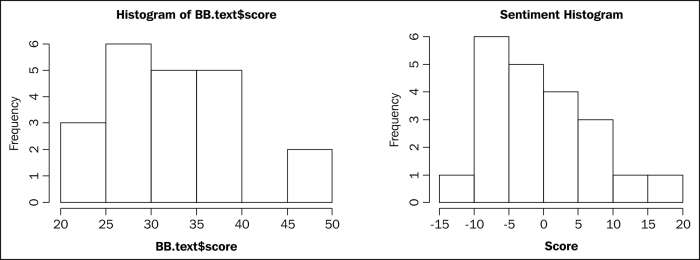
Histogram of BB.sentiment$score and BBsentiment$meancenter
Some of the upcoming plots will use a package named ggplot2, created by Hadley Wickham. Though difficult to master, ggplot2 offers some rather elegant and powerful graphing. This package is different from the package used for plotting in Chapter 2, Getting Started with R, and is shown here to offer diversity in the ways in which you may plot graphics. There are some rather good resources available if you are interested in learning more about ggplot2, but The Grammar of Graphics by Leland Wilkinson may be the most comprehensive:
# install and load ggplot2
install.packages("ggplot2")
require(ggplot2)
# using the results from the function to score our documents we create
# a boxplot to examine the distribution of opinion relating to
# economic conditions the labeling assumes here that you imported
# summary file of three years
> BB.boxplot<- ggplot(BB.sentiment, aes(x = BB.sentiment$year,
  y = BB.sentiment$centered, group = BB.text$year))+
  > geom_boxplot(aes(fill = BB.sentiment$year),
  outlier.colour = "black", outlier.shape = 16, outlier.size = 2)
# add labels to our boxplot using xlab ("Year"), ylab("Sentiment(Centered)"), and ggtitle             # ("Economic Sentiment - Beige Book (2011-2013)")
> BB.boxplot<- BB.boxplot + xlab("Year") + ylab("Sentiment (Centered)") +
  ggtitle("Economic Sentiment - Beige Book (2011-2013)")
# draw boxplot
BB.boxplot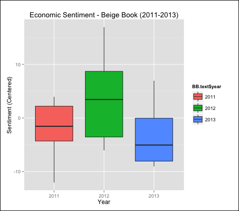
BB.boxplot
This simple example exposes some interesting insight into the economic conditions in the United States as reflected by the Beige Book. The x axis shows year and the y axis reflects mean-centered sentiment. Immediately, we can see that both 2011 and 2013 were below the mean sentiment over the entire document space (with the mean of 2013 below that of 2011). The boxplot shows us that while 2012 was above the mean, it had quite a bit of variability as reflected by the large interquartile range. We can also use this visualization to make comparisons between years—note that 2011 has a higher median value than 2013 but also has lower values as shown by the lower hinge. We can also reduce the data to month-by-year instead of merely year to potentially expose further patterns and increased variability. The following boxplot uses a larger portion of the data and reflects the ups and downs of sentiment over time:
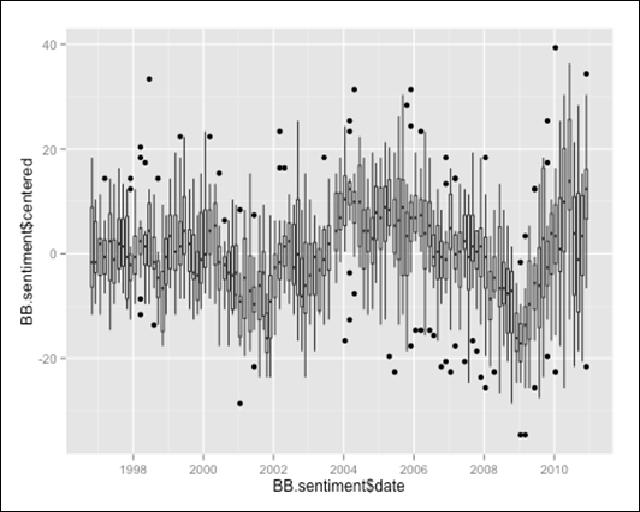
BB.boxplot
The screenshot after the following example shows economic sentiment with recession bars highlighted (2001-2002, 2007-2009):
# this code can be used to add the recession bars shown below where xmin and xmax    # are used to add vertical columns to our plot.
> rect2001 <- data.frame (
  xmin=2001, xmax=2002, ymin=-Inf, ymax=Inf)
> rect2007 <- data.frame (
  xmin=2007, xmax=2009, ymin=-Inf, ymax=Inf)

# ggplot is an R package used for advanced plotting.
> BB.boxplot <- ggplot(BB.sentiment, aes(x=BB.sentiment$year, y=BB.sentiment$centered,    group=BB.sentiment$year))
> BB.boxplot <- BB.boxplot + geom_boxplot(outlier.colour = "black",
     outlier.shape = 16, outlier.size = 2)
> BB.boxplot <- BB.boxplot + geom_rect(data=rect2001, aes(xmin=xmin,
     xmax=xmax, ymin=-Inf, ymax=+Inf), fill='pink', alpha=0.2, inherit.aes = FALSE)
> BB.boxplot <- BB.boxplot + geom_rect(data=rect2007, aes(xmin=xmin,
     xmax=xmax, ymin=-Inf, ymax=+Inf), fill='pink', alpha=0.2, inherit.aes = FALSE)
> BB.boxplot <- BB.boxplot + xlab("Date") + ylab("Sentiment
     (Centered)") + ggtitle("Economic Sentiment - Beige Book (1996-2010)")
> BB.boxplot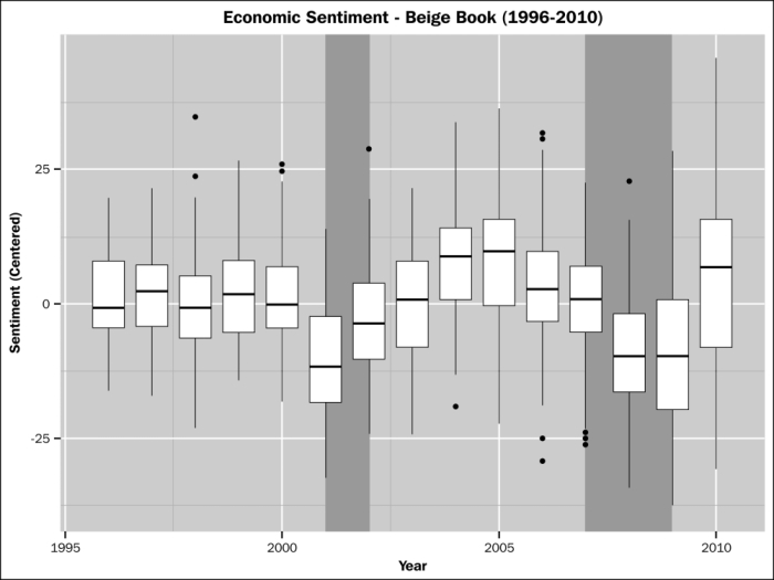
Boxplots with recession bars