
5.5 Compilation Techniques
Even though we don’t write our own assembly code much of the time, we still care about the characteristics of the code our compiler generates: its speed, its size, and its power consumption. Understanding how a compiler works will help us write code and direct the compiler to get the assembly language implementation we want. We will start with an overview of the compilation process, then some basic compilation methods, and conclude with some more advanced optimizations.
5.5.1 The Compilation Process
It is useful to understand how a high-level language program is translated into instructions: interrupt handling instructions, placement of data and instructions in memory, etc. Understanding how the compiler works can help you know when you cannot rely on the compiler. Next, because many applications are also performance sensitive, understanding how code is generated can help you meet your performance goals, either by writing high-level code that gets compiled into the instructions you want or by recognizing when you must write your own assembly code.
We can summarize the compilation process with a formula:
![]()
The high-level language program is translated into the lower-level form of instructions; optimizations try to generate better instruction sequences than would be possible if the brute force technique of independently translating source code statements were used. Optimization techniques focus on more of the program to ensure that compilation decisions that appear to be good for one statement are not unnecessarily problematic for other parts of the program.
The compilation process is outlined in Figure 5.13. Compilation begins with high-level language code such as C or C++ and generally produces assembly code. (Directly producing object code simply duplicates the functions of an assembler, which is a very desirable stand-alone program to have.) The high-level language program is parsed to break it into statements and expressions. In addition, a symbol table is generated, which includes all the named objects in the program. Some compilers may then perform higher-level optimizations that can be viewed as modifying the high-level language program input without reference to instructions.
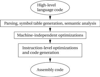
Figure 5.13 The compilation process.
Simplifying arithmetic expressions is one example of a machine-independent optimization. Not all compilers do such optimizations, and compilers can vary widely regarding which combinations of machine-independent optimizations they do perform. Instruction-level optimizations are aimed at generating code. They may work directly on real instructions or on a pseudo-instruction format that is later mapped onto the instructions of the target CPU. This level of optimization also helps modularize the compiler by allowing code generation to create simpler code that is later optimized. For example, consider this array access code:
x[i] = c*x[i];
A simple code generator would generate the address for x[i] twice, once for each appearance in the statement. The later optimization phases can recognize this as an example of common expressions that need not be duplicated. While in this simple case it would be possible to create a code generator that never generated the redundant expression, taking into account every such optimization at code generation time is very difficult. We get better code and more reliable compilers by generating simple code first and then optimizing it.
5.5.2 Basic Compilation Methods
Statement translation
In this section, we consider the basic job of translating the high-level language program with little or no optimization. Let’s first consider how to translate an expression. A large amount of the code in a typical application consists of arithmetic and logical expressions. Understanding how to compile a single expression, as described in the next example, is a good first step in understanding the entire compilation process.
Example 5.2 Compiling an Arithmetic Expression
Consider this arithmetic expression:
x = a*b + 5*(c − d)
The expression is written in terms of program variables. In some machines we may be able to perform memory-to-memory arithmetic directly on the locations corresponding to those variables. However, in many machines, such as the ARM, we must first load the variables into registers. This requires choosing which registers receive not only the named variables but also intermediate results such as (c − d).
The code for the expression can be built by walking the data flow graph. Here is the data flow graph for the expression.
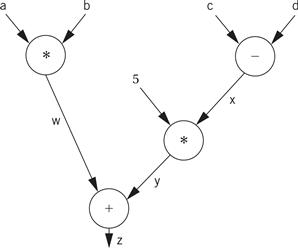
The temporary variables for the intermediate values and final result have been named w, x, y, and z. To generate code, we walk from the tree’s root (where z, the final result, is generated) by traversing the nodes in post order. During the walk, we generate instructions to cover the operation at every node. Here is the path:
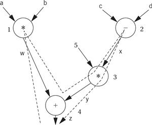
The nodes are numbered in the order in which code is generated. Because every node in the data flow graph corresponds to an operation that is directly supported by the instruction set, we simply generate an instruction at every node. Because we are making an arbitrary register assignment, we can use up the registers in order starting with r1. Here is the resulting ARM code:
; operator 1 (+)
ADR r4,a ; get address for a
MOV r1,[r4] ; load a
ADR r4,b ; get address for b
MOV r2,[r4] ; load b
ADD r3,r1,r2 ; put w into r3
; operator 2 (−)
ADR r4,c ; get address for c
MOV r4,[r4] ; load c
ADR r4,d ; get address for d
MOV r5,[r4] ; load d
SUB r6,r4,r5 ; put z into r6
; operator 3 (*)
MUL r7,r6,#5 ; operator 3, puts y into r7
; operator 4 (+)
ADD r8,r7,r3 ; operator 4, puts x into r8
; assign to x
ADR r1,x
STR r8,[r1] ; assigns to x location
One obvious optimization is to reuse a register whose value is no longer needed. In the case of the intermediate values w, y, and z, we know that they cannot be used after the end of the expression (e.g., in another expression) because they have no name in the C program. However, the final result z may in fact be used in a C assignment and the value reused later in the program. In this case we would need to know when the register is no longer needed to determine its best use.
For comparison, here is the code generated by the ARM gcc compiler with handwritten comments:
ldr r2, [fp, #−16]
ldr r3, [fp, #−20]
mul r1, r3, r2 ; multiply
ldr r2, [fp, #−24]
ldr r3, [fp, #−28]
rsb r2, r3, r2 ; subtract
mov r3, r2
mov r3, r3, asl #2
add r3, r3, r2 ; add
add r3, r1, r3 ; add
str r3, [fp, #−32] ; assign
In the previous example, we made an arbitrary allocation of variables to registers for simplicity. When we have large programs with multiple expressions, we must allocate registers more carefully because CPUs have a limited number of registers. We will consider register allocation in more detail below.
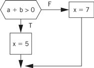
We also need to be able to translate control structures. Because conditionals are controlled by expressions, the code generation techniques of the last example can be used for those expressions, leaving us with the task of generating code for the flow of control itself. Figure 5.14 shows a simple example of changing flow of control in C—an if statement, in which the condition controls whether the true or false branch of the if is taken. Figure 5.14 also shows the control flow diagram for the if statement.
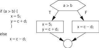
Figure 5.14 Flow of control in C and control flow diagrams.
The next example illustrates how to implement conditionals in assembly language.
Example 5.3 Generating Code for a Conditional
Consider this C statement:
if (a + b > 0)
x = 5;
else
x = 7;
The CDFG for the statement appears below.
We know how to generate the code for the expressions. We can generate the control flow code by walking the CDFG. One ordered walk through the CDFG follows:
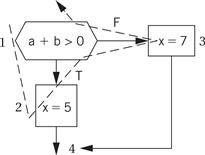
To generate code, we must assign a label to the first instruction at the end of a directed edge and create a branch for each edge that does not go to the immediately following instruction. The exact steps to be taken at the branch points depend on the target architecture. On some machines, evaluating expressions generates condition codes that we can test in subsequent branches, and on other machines we must use test-and-branch instructions. ARM allows us to test condition codes, so we get the following ARM code for the 1-2-3 walk:
ADR r5,a ; get address for a
LDR r1,[r5] ; load a
ADR r5,b ; get address for b
LDR r2,b ; load b
ADD r3,r1,r2
BLE label3 ; true condition falls through branch
; true case
LDR r3,#5 ; load constant
ADR r5,x
STR r3, [r5] ; store value into x
B stmtend ; done with the true case
; false case
label3 LDR r3,#7 ; load constant
ADR r5,x ; get address of x
STR r3,[r5] ; store value into x
stmtend …
The 1-2 and 3-4 edges do not require a branch and label because they are straight-line code. In contrast, the 1-3 and 2-4 edges do require a branch and a label for the target.
For comparison, here is the code generated by the ARM gcc compiler with some handwritten comments:
ldr r2, [fp, #−16]
ldr r3, [fp, #−20]
add r3, r2, r3
cmp r3, #0 ; test the branch condition
ble .L3 ; branch to false block if < =
mov r3, #5 ; true block
str r3, [fp, #−32]
b .L4 ; go to end of if statement
.L3: ; false block
mov r3, #7
str r3, [fp, #−32]
.L4:
Because expressions are generally created as straight-line code, they typically require careful consideration of the order in which the operations are executed. We have much more freedom when generating conditional code because the branches ensure that the flow of control goes to the right block of code. If we walk the CDFG in a different order and lay out the code blocks in a different order in memory, we still get valid code as long as we properly place branches.
Drawing a control flow graph based on the while form of the loop helps us understand how to translate it into instructions.
C compilers can generate (using the -s flag) assembler source, which some compilers intersperse with the C code. Such code is a very good way to learn about both assembly language programming and compilation.
Procedures
Another major code generation problem is the creation of procedures. Generating code for procedures is relatively straightforward once we know the procedure linkage appropriate for the CPU. At the procedure definition, we generate the code to handle the procedure call and return. At each call of the procedure, we set up the procedure parameters and make the call.
The CPU’s subroutine call mechanism is usually not sufficient to directly support procedures in modern programming languages. We introduced the procedure stack and procedure linkages in Chapter 2. The linkage mechanism provides a way for the program to pass parameters into the program and for the procedure to return a value. It also provides help in restoring the values of registers that the procedure has modified. All procedures in a given programming language use the same linkage mechanism (although different languages may use different linkages). The mechanism can also be used to call handwritten assembly language routines from compiled code.
Procedure stacks are typically built to grow down from high addresses. A stack pointer (sp) defines the end of the current frame, while a frame pointer (fp) defines the end of the last frame. (The fp is technically necessary only if the stack frame can be grown by the procedure during execution.) The procedure can refer to an element in the frame by addressing relative to sp. When a new procedure is called, the sp and fp are modified to push another frame onto the stack.
As we saw in Chapter 2, the ARM Procedure Call Standard (APCS) [Slo04] is the recommended procedure linkage for ARM processors. r0–r3 are used to pass the first four parameters into the procedure. r0 is also used to hold the return value.
The next example looks at compiler-generated procedure linkage code.
Example 5.4 Procedure Linkage in C
Here is a procedure definition:
int p1(int a, int b, int c, int d, int e) {
return a + e;
}
This procedure has five parameters, so we would expect that one of them would be passed through the stack while the rest are passed through registers. It also returns an integer value, which should be returned in r0. Here is the code for the procedure generated by the ARM gcc compiler with some handwritten comments:
mov ip, sp ; procedure entry
stmfd sp!, {fp, ip, lr, pc}
sub fp, ip, #4
sub sp, sp, #16
str r0, [fp, #−16] ; put first four args on stack
str r1, [fp, #−20]
str r2, [fp, #−24]
str r3, [fp, #−28]
ldr r2, [fp, #−16] ; load a
ldr r3, [fp, #4] ; load e
add r3, r2, r3 ; compute a + e
mov r0, r3 ; put the result into r0 for return
ldmea fp, {fp, sp, pc} ; return
Here is a call to that procedure:
y = p1(a,b,c,d,x);
Here is the ARM gcc code with handwritten comments:
ldr r3, [fp, #−32] ; get e
str r3, [sp, #0] ; put into p1()’s stack frame
ldr r0, [fp, #−16] ; put a into r0
ldr r1, [fp, #−20] ; put b into r1
ldr r2, [fp, #−24] ; put c into r2
ldr r3, [fp, #−28] ; put d into r3
bl p1 ; call p1()
mov r3, r0 ; move return value into r3
str r3, [fp, #−36] ; store into y in stack frame
We can see that the compiler sometimes makes additional register moves but it does follow the ACPS standard.
Data structures
The compiler must also translate references to data structures into references to raw memories. In general, this requires address computations. Some of these computations can be done at compile time while others must be done at run time.
Arrays are interesting because the address of an array element must in general be computed at run time, because the array index may change. Let us first consider a one-dimensional array:
a[i]
The layout of the array in memory is shown in Figure 5.15: the zeroth element is stored as the first element of the array, the first element directly below, and so on. We can create a pointer for the array that points to the array’s head, namely, a[0]. If we call that pointer aptr for convenience, then we can rewrite the reading of a[i] as
*(aptr + i)
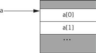
Figure 5.15 Layout of a one-dimensional array in memory.
Two-dimensional arrays are more challenging. There are multiple possible ways to lay out a two-dimensional array in memory, as shown in Figure 5.15. In this form, which is known as row major, the inner variable of the array (j in a[i,j]) varies most quickly. (Fortran uses a different organization known as column major.) Two-dimensional arrays also require more sophisticated addressing—in particular, we must know the size of the array. Let us consider the row-major form. If the a[] array is of size N × M, then we can turn the two-dimensional array access into a one-dimensional array access. Thus,
a[i,j]
becomes
a[i*M + j]
where the maximum value for j is M − 1.
A C struct is easier to address. As shown in Figure 5.16, a structure is implemented as a contiguous block of memory. Fields in the structure can be accessed using constant offsets to the base address of the structure. In this example, if field1 is four bytes long, then field2 can be accessed as
*(aptr + 4)
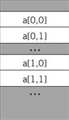
Figure 5.16 Memory layout for two-dimensional arrays.
This addition can usually be done at compile time, requiring only the indirection itself to fetch the memory location during execution.
5.5.3 Compiler Optimizations
Basic compilation techniques can generate inefficient code. Compilers use a wide range of algorithms to optimize the code they generate.
Loop transformations
Loops are important program structures—although they are compactly described in the source code, they often use a large fraction of the computation time. Many techniques have been designed to optimize loops.
A simple but useful transformation is known as loop unrolling, illustrated in the next example. Loop unrolling is important because it helps expose parallelism that can be used by later stages of the compiler.
Example 5.5 Loop Unrolling
Here is a simple C loop:
for (i = 0; i < N; i++) {
a[i]=b[i]*c[i];
}
This loop is executed a fixed number of times, namely, N. A straightforward implementation of the loop would create and initialize the loop variable i, update its value on every iteration, and test it to see whether to exit the loop. However, because the loop is executed a fixed number of times, we can generate more direct code.
If we let N = 4, then we can substitute this straight-line code for the loop:
a[0] = b[0]*c[0];
a[1] = b[1]*c[1];
a[2] = b[2]*c[2];
a[3] = b[3]*c[3];
This unrolled code has no loop overhead code at all, that is, no iteration variable and no tests. But the unrolled loop has the same problems as the inlined procedure—it may interfere with the cache and expands the amount of code required.
We do not, of course, have to fully unroll loops. Rather than unroll the above loop four times, we could unroll it twice. Unrolling produces this code:
for (i = 0; i < 2; i++) {
a[i*2] = b[i*2]*c[i*2];
a[i*2 + 1] = b[i*2 + 1]*c[i*2 + 1];
}
In this case, because all operations in the two lines of the loop body are independent, later stages of the compiler may be able to generate code that allows them to be executed efficiently on the CPU’s pipeline.
Loop fusion combines two or more loops into a single loop. For this transformation to be legal, two conditions must be satisfied. First, the loops must iterate over the same values. Second, the loop bodies must not have dependencies that would be violated if they are executed together—for example, if the second loop’s ith iteration depends on the results of the i + 1th iteration of the first loop, the two loops cannot be combined. Loop distribution is the opposite of loop fusion, that is, decomposing a single loop into multiple loops.
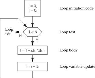
Loop tiling breaks up a loop into a set of nested loops, with each inner loop performing the operations on a subset of the data. An example is shown in Figure 5.17. Here, each loop is broken up into tiles of size two. Each loop is split into two loops—for example, the inner ii loop iterates within the tile and the outer i loop iterates across the tiles. The result is that the pattern of accesses across the a array is drastically different—rather than walking across one row in its entirety, the code walks through rows and columns following the tile structure. Loop tiling changes the order in which array elements are accessed, thereby allowing us to better control the behavior of the cache during loop execution.
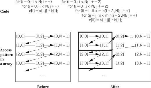
Figure 5.17 Loop tiling.
We can also modify the arrays being indexed in loops. Array padding adds dummy data elements to a loop in order to change the layout of the array in the cache. Although these array locations will not be used, they do change how the useful array elements fall into cache lines. Judicious padding can in some cases significantly reduce the number of cache conflicts during loop execution.
Dead code elimination
Dead code is code that can never be executed. Dead code can be generated by programmers, either inadvertently or purposefully. Dead code can also be generated by compilers. Dead code can be identified by reachability analysis—finding the other statements or instructions from which it can be reached. If a given piece of code cannot be reached, or it can be reached only by a piece of code that is unreachable from the main program, then it can be eliminated. Dead code elimination analyzes code for reachability and trims away dead code.
Register allocation
Register allocation is a very important compilation phase. Given a block of code, we want to choose assignments of variables (both declared and temporary) to registers to minimize the total number of required registers.
The next example illustrates the importance of proper register allocation.
Example 5.6 Register Allocation
To keep the example small, we assume that we can use only four of the ARM’s registers. In fact, such a restriction is not unthinkable—programming conventions can reserve certain registers for special purposes and significantly reduce the number of general-purpose registers available.
Consider this C code:
w = a + b; /* statement 1 */
x = c + w; /* statement 2 */
y = c + d; /* statement 3 */
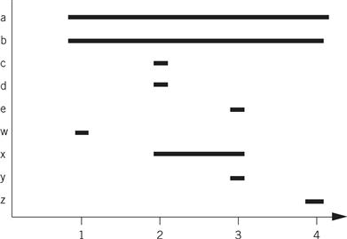
A naive register allocation, assigning each variable to a separate register, would require seven registers for the seven variables in the above code. However, we can do much better by reusing a register once the value stored in the register is no longer needed. To understand how to do this, we can draw a lifetime graph that shows the statements on which each statement is used. Here is a lifetime graph in which the x axis is the statement number in the C code and the y axis shows the variables.
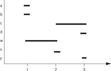
A horizontal line stretches from the first statement where the variable is used to the last use of the variable; a variable is said to be live during this interval. At each statement, we can determine every variable currently in use. The maximum number of variables in use at any statement determines the maximum number of registers required. In this case, statement two requires three registers: c, w, and x. This fits within the four-register limitation. By reusing registers once their current values are no longer needed, we can write code that requires no more than four registers. Here is one register assignment:
| a | r0 |
| b | r1 |
| c | r2 |
| d | r0 |
| w | r3 |
| x | r0 |
| y | r3 |
Here is the ARM assembly code that uses the above register assignment:
LDR r0,[p_a] ; load a into r0 using pointer to a (p_a)
LDR r1,[p_b] ; load b into r1
ADD r3,r0,r1 ; compute a + b
STR r3,[p_w] ; w = a + b
LDR r2,[p_c] ; load c into r2
ADD r0,r2,r3 ; compute c + w, reusing r0 for x
STR r0,[p_x] ; x = c + w
LDR r0,[p_d] ; load d into r0
ADD r3,r2,r0 ; compute c + d, reusing r3 for y
STR r3,[p_y] ; y = c + d
If a section of code requires more registers than are available, we must spill some of the values out to memory temporarily. After computing some values, we write the values to temporary memory locations, reuse those registers in other computations, and then reread the old values from the temporary locations to resume work. Spilling registers is problematic in several respects: it requires extra CPU time and uses up both instruction and data memory. Putting effort into register allocation to avoid unnecessary register spills is worth your time.
We can solve register allocation problems by building a conflict graph and solving a graph coloring problem. As shown in Figure 5.18, each variable in the high-level language code is represented by a node. An edge is added between two nodes if they are both live at the same time. The graph coloring problem is to use the smallest number of distinct colors to color all the nodes such that no two nodes are directly connected by an edge of the same color. The figure shows a satisfying coloring that uses three colors. Graph coloring is NP-complete, but there are efficient heuristic algorithms that can give good results on typical register allocation problems.
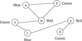
Figure 5.18 Using graph coloring to solve the problem of Example 5.6.
Lifetime analysis assumes that we have already determined the order in which we will evaluate operations. In many cases, we have freedom in the order in which we do things. Consider this expression:
(a + b) * (c − d)
We have to do the multiplication last, but we can do either the addition or the subtraction first. Different orders of loads, stores, and arithmetic operations may also result in different execution times on pipelined machines. If we can keep values in registers without having to reread them from main memory, we can save execution time and reduce code size as well.
The next example shows how proper operator scheduling can improve register allocation.
Example 5.7 Operator Scheduling for Register Allocation
Here is a sample C code fragment:
w = a + b; /* statement 1 */
x = c + d; /* statement 2 */
y = x + e; /* statement 3 */
z = a − b; /* statement 4 */
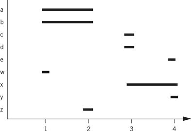
If we compile the statements in the order in which they were written, we get this register graph:
Because w is needed until the last statement, we need five registers at statement 3, even though only three registers are needed for the statement at line 3. If we swap statements 3 and 4 (renumbering them 39 and 49), we reduce our requirements to three registers. Here is the modified C code:
w = a + b; /* statement 1 */
z = a − b; /* statement 29 */
x = c + d; /* statement 39 */
y = x + e; /* statement 49 */
And here is the lifetime graph for the new code:
Compare the ARM assembly code for the two code fragments. We have written both assuming that we have only four free registers. In the before version, we do not have to write out any values, but we must read a and b twice. The after version allows us to retain all values in registers as long as we need them.
Before version After version
LDR r0,a LDR r0,a
LDR r1,b LDR r1,b
ADD r2,r0,r1 ADD r2,r1,r0
STR r2,w ; w = a + b STR r2,w ; w = a + b
LDRr r0,c SUB r2,r0,r1
LDR r1,d STR r2,z ; z = a − b
ADD r2,r0,r1 LDR r0,c
STR r2,x ; x = c + d LDR r1,d
LDR r1,e ADD r2,r1,r0
ADD r0,r1,r2 STR r2,x ; x = c + d
STR r0,y ; y = x + e LDR r1,e
LDR r0,a ; reload a ADD r0,r1,r2
LDR r1,b ; reload b STR r0,y ; y = x + e
SUB r2,r1,r0
STR r2,z ; z = a − b
Scheduling
We have some freedom to choose the order in which operations will be performed. We can use this to our advantage—for example, we may be able to improve the register allocation by changing the order in which operations are performed, thereby changing the lifetimes of the variables.
We can solve scheduling problems by keeping track of resource utilization over time. We do not have to know the exact microarchitecture of the CPU—all we have to know is that, for example, instruction types 1 and 2 both use resource A while instruction types 3 and 4 use resource B. CPU manufacturers generally disclose enough information about the microarchitecture to allow us to schedule instructions even when they do not provide a detailed description of the CPU’s internals.
We can keep track of CPU resources during instruction scheduling using a reservation table[Kog81]. As illustrated in Figure 5.19, rows in the table represent instruction execution time slots and columns represent resources that must be scheduled. Before scheduling an instruction to be executed at a particular time, we check the reservation table to determine whether all resources needed by the instruction are available at that time. Upon scheduling the instruction, we update the table to note all resources used by that instruction. Various algorithms can be used for the scheduling itself, depending on the types of resources and instructions involved, but the reservation table provides a good summary of the state of an instruction scheduling problem in progress.

Figure 5.19 A reservation table for instruction scheduling.
We can also schedule instructions to maximize performance. As we know from Section 3.6, when an instruction that takes more cycles than normal to finish is in the pipeline, pipeline bubbles appear that reduce performance. Software pipelining is a technique for reordering instructions across several loop iterations to reduce pipeline bubbles. Some instructions take several cycles to complete; if the value produced by one of these instructions is needed by other instructions in the loop iteration, then they must wait for that value to be produced. Rather than pad the loop with no-ops, we can start instructions from the next iteration. The loop body then contains instructions that manipulate values from several different loop iterations—some of the instructions are working on the early part of iteration n + 1, others are working on iteration n, and still others are finishing iteration n − 1.
Instruction selection
Selecting the instructions to use to implement each operation is not trivial. There may be several different instructions that can be used to accomplish the same goal, but they may have different execution times. Moreover, using one instruction for one part of the program may affect the instructions that can be used in adjacent code. Although we can’t discuss all the problems and methods for code generation here, a little bit of knowledge helps us envision what the compiler is doing.
One useful technique for generating code is template matching, illustrated in Figure 5.20. We have a DAG that represents the expression for which we want to generate code. In order to be able to match up instructions and operations, we represent instructions using the same DAG representation. We shaded the instruction template nodes to distinguish them from code nodes. Each node has a cost, which may be simply the execution time of the instruction or may include factors for size, power consumption, and so on. In this case, we have shown that each instruction takes the same amount of time, and thus all have a cost of 1. Our goal is to cover all nodes in the code DAG with instruction DAGs—until we have covered the code DAG we haven’t generated code for all the operations in the expression. In this case, the lowest-cost covering uses the multiply-add instruction to cover both nodes. If we first tried to cover the bottom node with the multiply instruction, we would find ourselves blocked from using the multiply-add instruction. Dynamic programming can be used to efficiently find the lowest-cost covering of trees, and heuristics can extend the technique to DAGs.
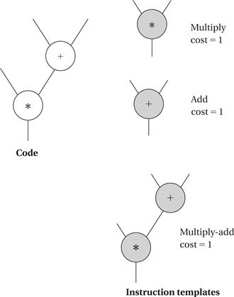
Figure 5.20 Code generation by template matching.
Understanding your compiler
Clearly, the compiler can vastly transform your program during the creation of assembly language. But compilers are also substantially different in terms of the optimizations they perform. Understanding your compiler can help you get the best code out of it.
Studying the assembly language output of the compiler is a good way to learn about what the compiler does. Some compilers will annotate sections of code to help you make the correspondence between the source and assembler output. Starting with small examples that exercise only a few types of statements will help. You can experiment with different optimization levels (the -O flag on most C compilers). You can also try writing the same algorithm in several ways to see how the compiler’s output changes.
If you can’t get your compiler to generate the code you want, you may need to write your own assembly language. You can do this by writing it from scratch or modifying the output of the compiler. If you write your own assembly code, you must ensure that it conforms to all compiler conventions, such as procedure call linkage. If you modify the compiler output, you should be sure that you have the algorithm right before you start writing code so that you don’t have to repeatedly edit the compiler’s assembly language output. You also need to clearly document the fact that the high-level language source is, in fact, not the code used in the system.