5.12.1 Theory of Operation and Requirements

In order to understand the digital still camera, we must first understand the digital photography process. A modern digital camera performs a great many steps:

In addition to actually taking the photo, the camera must perform several other important operations, often simultaneously with the picture-taking process. It must, for example, update the camera’s electronic display. It must also listen for button presses from the user, which may command operations that modify the current operation of the camera. The camera should also provide a browser with which the user can review the stored images.

Much of this terminology comes largely from film photography—for example, the decisions made while developing a digital photo are similar to those made in the development of a film image, even though the steps to carry out those decisions are very different. Many variations are possible on all of these steps but the basic process is common to all digital still cameras. A few basic terms are useful: the image is divided into pixels; a pixel’s brightness is often referred to as its luminance; a color pixel’s brightness in a particular color is known as chrominance.

The camera can use the image sensor data to drive the exposure-setting process. Several algorithms are possible but all involve starting with a test exposure and using some search algorithm to select the final exposure. Exposure-setting may also use any of several different metrics to judge the exposure. The simplest metric is the average luminance of a pixel. The camera may evaluate some function of several points in the image. It may also evaluate the image’s histogram. The histogram is composed by sorting the pixels into bins by luminance; 256 bins is a common choice for the resolution of the histogram. The histogram gives us more information than does a single average. For instance, we can tell whether many pixels are overexposed or underexposed by looking at the bins at the extremes of luminance.

Three major approaches are used to determine focus: active rangefinding, phase detection, contrast detection. Active rangefinding uses a pulse that is sent out and the time-of-flight of the reflected and returned pulse is measured to determine distance. Ultrasound was used in one early autofocus system, the Polaroid SX-70, but today infrared pulses are more commonly used. Phase detection compares light from opposite sides of the lens, creating an optical rangefinder. Contrast detection relies on the fact that out-of-focused edges do not display the sharp changes in luminance of in-focus edges. The simplest algorithms for contrast detection evaluate focus at pre-determined points in the image, which may require the photographer to move the camera to place a suitable edge at one of the autofocus spots.

Two major types of image sensors are used in modern cameras [Nak05]: charged-coupled devices (CCDs) and CMOS. For our purposes, the operation of these two in a digital still camera are equivalent.

Developing the image involves both putting the image in usable form and improving its quality. The most basic operation required for a color image is to interpolate a full color value for each pixel. Most image sensors capture color images using a color filter array—color filters that cover a single pixel. The filters usually capture one of the primary colors—red, green, and blue—and are arranged in a two-dimensional pattern. The first such color filter array was proposed by Bayer [Bay76]. His pattern is still widely used and known as the Bayer pattern. As shown in Figure 5.35, the Bayer pattern is a 2 × 2 array with two green, one blue, and one red pixels. More green pixels are used because the eye is most sensitive to green, which Bayer viewed as a simple luminance signal. Because each image sensor pixel captured only one of the primaries, the other two primaries must be interpolated for each pixel. This process is known as Bayer pattern interpolation or demosaicing. The simplest interpolation algorithm is a simple average, which can also be used as a low-pass filter. For example, we can interpolate the missing values from the green pixel G2.1 as:

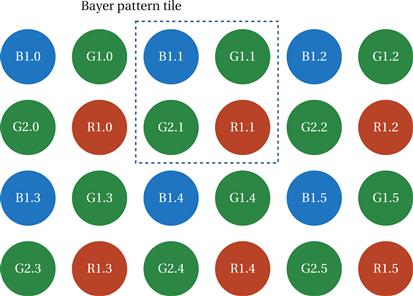
Figure 5.35 A color filter array arranged in a Bayer pattern.

We can use more information to interpolate missing green values. For example, the green value associated with red pixel R1.1 can be interpolated from the four nearest green pixels:

However, this simple interpolation algorithm introduces color fringes at edges. More sophisticated interpolation algorithms exist to minimize color fringing while maintaining other aspects of image quality.

Development also determines and corrects for color temperature in the scene. Different light sources can be composed of light of different colors; color can be described as the temperature of a black body that will emit radiation of that frequency. The human visual system automatically corrects for color temperature. We do not, for example, notice that fluorescent lights emit a greenish cast. However, a photo taken without color temperature correction will display a cast from the color of light used to illuminate the scene. A variety of algorithms exist to determine the color temperature. A set of chrominance histograms is often used to judge color temperature. Once a color correction is determined, it can be applied to the pixels in the image.

Many cameras also apply sharpening algorithms to reduce some of the effects of pixellation in digital image capture. Once again, a variety of sharpening algorithms are used. These algorithms apply filters to sets of adjacent pixels.

Some cameras offer a RAW mode of image capture. The resulting RAW file holds the pixel values without processing. RAW capture allows the user to develop the image manually and offline using sophisticated algorithms and programs. Although generic RAW file formats exist, most camera manufacturers use proprietary RAW formats. Some uncompressed image formats also exist, such as TIFF [Ado92].

Compression reduces the amount of storage required for the image. Some lossless compression methods are used that do not throw away information from the image. However, most images are stored using lossy compression. A lossy compression algorithm throws away information in the image, so that the decompression process cannot reproduce an exact copy of the original image. A number of compression techniques have been developed to substantially reduce the storage space required for an image without noticeably affecting image quality. The most common family of compression algorithms is JPEG[CCI92]. (JPEG stands for Joint Photographic Experts Group.) The JPEG standard was extended as JPEG 2000 but classic JPEG is still widely used. The JPEG standard itself contains a large number of options, not all of which need to be implemented to conform to the standard.

As shown in Figure 5.36, the typical compression process used for JPEG images has five main steps:

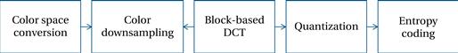
Figure 5.36 The typical JPEG compression process.

(We call this typical because the standard allows for several variations.) The first step puts the color image into a form that allows optimizations less likely to reduce image quality. Color can be represented by a number of color spaces or combinations of colors that, when combined, form the full range of colors. We saw the red/green/blue (RGB) color space in the color filter array. For compression, we convert to the Y’C_RC_B color space: Y’ is a luminance channel, C_R is a red channel, and C_B is a blue channel. The conversion between these two color spaces is defined by the JFIF standard [Ham92]:

Once in Y’C_RC_B form, the C_R and C_B is generally reduced by downsampling. The 4:2:2 method downsamples both C_R and C_B to half their normal resolution only in the horizontal direction. The 4:2:0 method downsamples both C_R and C_B both horizontally and vertically. Downsampling reduces the amount of data required and is justified by the human visual system’s lower acuity in chrominance. The three color channels, Y’, C_R , and C_B , are processed separately.

The color channels are next separately broken into 8 × 8 blocks (the term block specifically refers to an 8 × 8 array of values in JPEG). The discrete cosine transform is applied to each block. DCT is a frequency transform that produces an 8 × 8 block of transform coefficients. It is reversible, so that the original values can be reconstructed from the transform coefficients. DCT does not itself reduce the amount of information in a block. Many highly optimized algorithms exist to compute the DCT, and in particular an 8 × 8 DCT.

The lossiness of the compression process occurs in the quantization step. This step changes the DCT coefficients with the aim to do so in a way that allows them to be stored in fewer bits. Quantization is applied on the DCT rather than on the pixels because some image characteristics are easier to identify in the DCT representation. Specifically, because the DCT breaks up the block according to spatial frequencies, quantization often reduces the high frequency content of the block. This strategy tends to significantly reduce the data set size during compression while causing less noticeable visual artifacts.

The quantization is defined by an 8 × 8 quantization matrix Q. A DCT coefficient G_i,j is quantized to a value B_i,j using the Q_i,j value from the quantization matrix:

The JPEG standard allows for different quantization matrices but gives a typical matrix that is widely used:

This matrix tends to zeroes in the lower-right coefficients. Higher spatial frequencies (and therefore finer detail) are represented by the coefficients in the lower and right parts of the matrix. Putting these to zero eliminates some fine detail from the block.

Quantization does not directly provide for a smaller representation of the image. Entropy coding (lossless encoding) recodes the quantized blocks in a form that requires fewer bits. JPEG allows multiple entropy coding algorithms to be used. The most common algorithm is Huffman coding. The encoding can be represented as a table that maps a fixed number of bits into a variable number of bits. This step encodes the difference between the current coefficient and the previous coefficient, not the coefficient itself. Several different styles of encoding are possible: baseline sequential codes one block at a time; baseline progressive encodes corresponding coefficients of every block.

Coefficients are read from the coefficient matrix in the zig-zag pattern shown in Figure 5.37. This pattern reads along diagonals from the upper left to the lower right, which corresponds to reading from lowest spatial frequency to highest spatial frequency. If fine detail is reduced equally in both horizontal and vertical dimensions, then zero coefficients are also arranged diagonally. The zig-zag pattern increases the length of sequences of zero coefficients in such cases. Long strings of zeroes can be coded in a very small number of bits.

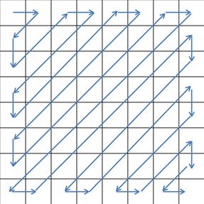
Figure 5.37 Zig-zag pattern for reading coefficients.

The requirements for the digital still camera are given in Figure 5.38.

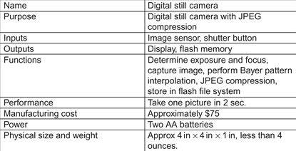
Figure 5.38 Requirements for the digital still camera.

5.12.2 Specification

A digital still camera must comply with a number of standards. These standards generally govern the format of output generated by the camera. Standards in general allow for some freedom of implementation in certain aspects while still adhering to the standard.

The Tagged Image File Format (TIFF) [Ado92] is often used to store uncompressed images, although it also supports several compression methods as well. Baseline TIFF specifies a basic format that also provides flexibility on image size, bits per pixel, compression, and other aspects of image storage.

The JPEG standard itself allows a number of options that can be followed in various combinations. A set of operations used to generate a compressed image is known as a process. The JFIF standard [Ham92] is a widely used file interchange format. It is compatible with the JPEG standard but specifies a number of items in more detail.

The Exchangeable Image File Format (EXIF) standard is widely used to further extend the information stored in an image file. As shown in Figure 5.39, an EXIF file holds several types of data:

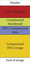
Figure 5.39 Structure of an EXIF file.

The entire image storage process is defined by yet another standard, the Design rule for Camera File (DCF) standard [CIP10]. DCF specifies three major steps: JPEG compression, EXIF file generation, and DOS FAT image storage. DCF specifies a number of aspects of file storage:

The Digital Print Order Format (DPOF) standard [DPO00] provides a standard way for camera users to order prints of selected photographs. Print orders can be captured in the camera, a home computer, or other devices and transmitted to a photofinisher or printer.

Even a simple point-and-shoot camera provides a number of options and modes. Two basic operations are fundamental: display a live view of the current image and capture an image.

Figure 5.40 shows a state diagram for the display. In normal operation, the camera repeatedly displays the latest image from the image sensor. After an image is captured, it is briefly shown on the display.

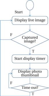
Figure 5.40 State diagram for display operation.

Figure 5.41 shows a state diagram for the picture-taking process. Depressing the shutter button half-way signals the camera to evaluate exposure and focus. Once the shutter is fully depressed, the image is captured, developed, compressed, and stored.

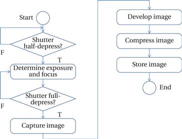
Figure 5.41 State diagram for picture taking.

5.12.3 System Architecture

The basic architecture of a digital still camera uses a controller to provide the basic sequencing for picture taking and camera operation. The controller calls on a number of other units to perform the various steps in each process.

Figure 5.42 shows the basic classes in a digital still camera. The controller class implements the state diagrams for camera operation. The buttons and display classes provide an abstraction of the physical user interface. The image sensor abstracts the operation of the sensor. The picture developer provides algorithms for mosaicing, sharpening, etc. The compression unit generates compressed image data. The file generator takes care of aspects of the file generation beyond compression. The file system performs basic file functions. Cameras may also provide other communication ports such as USB or Firewire.

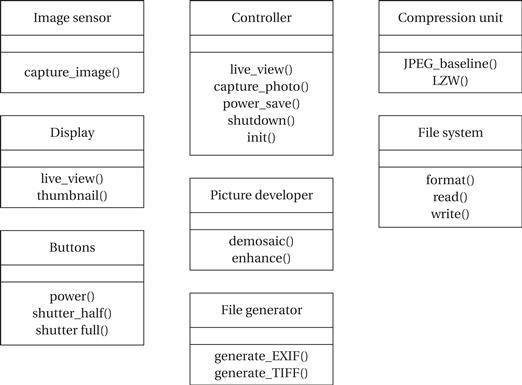
Figure 5.42 Basic classes in the digital still camera.

Figure 5.43 shows a typical block diagram for digital still camera hardware. While some cameras will use the same processor for both system control and image processing, many cameras rely on separate processors for these two tasks. The DSP may be programmable or custom hardware.

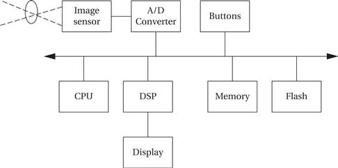
Figure 5.43 Computing platform for a digital still camera.

A sequence diagram for taking a photo is shown in Figure 5.44. This sequence diagram maps the basic operations onto the units in the hardware architecture.

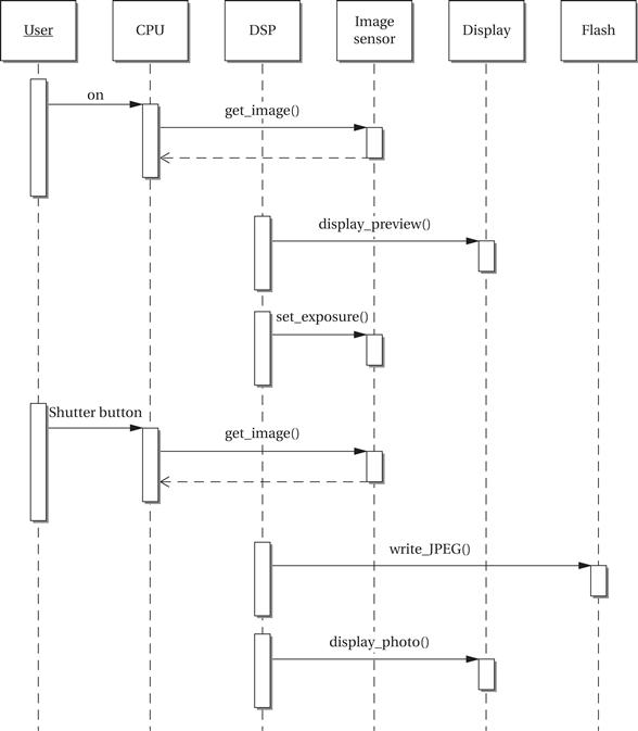
Figure 5.44 Sequence diagram for taking a picture with a digital still camera.

The design of buffering is very important in a digital still camera. Buffering affects the rate at which pictures can be taken, the energy consumed, and the cost of the camera. The image exists in several versions at different points in the process: the raw image from the image sensor; the developed image; the compressed image data; and the file. Most of this data is buffered in system RAM. However, displays may have their own memory to ensure adequate performance.

5.12.4 Component Design and Testing

Components based on standards, such as JPEG or FAT, may be implemented using modules developed elsewhere. JPEG compression in particular may be implemented with special-purpose hardware. DCT accelerators are common. Some digital still camera engines use hardware units that produce a complete JFIF file from an image.

The multiple buffering points in the picture taking process can help to simplify testing. Test file inputs can be introduced into the buffer by test scaffolding, then run with results in the output buffer checked against reference output.

5.12.5 System Integration and Testing

Buffers help to simplify system integration, although care must be taken to ensure that the buffers do not overlap in main memory.

Some tests can be performed by substituting pixel value streams for the sensor data. Final tests should make use of a target image so that qualities such as sharpness and color fidelity can be judged.