6.3 Multirate Systems
Implementing code that satisfies timing requirements is even more complex when multiple rates of computation must be handled. Multirate embedded computing systems are very common, including automobile engines, printers, and cell phones. In all these systems, certain operations must be executed periodically, and each operation is executed at its own rate.
Application Example 6.1 describes why automobile engines require multirate control.
Application Example 6.1 Automotive Engine Control
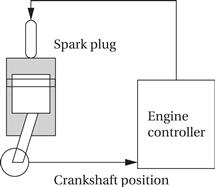
The simplest automotive engine controllers, such as the ignition controller for a basic motorcycle engine, perform only one task—timing the firing of the spark plug, which takes the place of a mechanical distributor. The spark plug must be fired at a certain point in the combustion cycle, but to obtain better performance, the phase relationship between the piston’s movement and the spark should change as a function of engine speed. Using a microcontroller that senses the engine crankshaft position allows the spark timing to vary with engine speed. Firing the spark plug is a periodic process (but note that the period depends on the engine’s operating speed).
The control algorithm for a modern automobile engine is much more complex, making the need for microprocessors that much greater. Automobile engines must meet strict requirements (mandated by law in the United States) on both emissions and fuel economy. On the other hand, the engines must still satisfy customers not only in terms of performance but also in terms of ease of starting in extreme cold and heat, low maintenance, and so on.
Automobile engine controllers use additional sensors, including the gas pedal position and an oxygen sensor used to control emissions. They also use a multimode control scheme. For example, one mode may be used for engine warm-up, another for cruise, and yet another for climbing steep hills, and so forth. The larger number of sensors and modes increases the number of discrete tasks that must be performed. The highest-rate task is still firing the spark plugs. The throttle setting must be sampled and acted upon regularly, although not as frequently as the crankshaft setting and the spark plugs. The oxygen sensor responds much more slowly than the throttle, so adjustments to the fuel/air mixture suggested by the oxygen sensor can be computed at a much lower rate.
The engine controller takes a variety of inputs that determine the state of the engine. It then controls two basic engine parameters: the spark plug firings and the fuel/air mixture. The engine control is computed periodically, but the periods of the different inputs and outputs range over several orders of magnitude of time. An early paper on automotive electronics by Marley [Mar78] described the rates at which engine inputs and outputs must be handled:
| Variable | Time to move full | Update period (ms) |
| Engine spark timing | 300 | 2 |
| Throttle | 40 | 2 |
| Air flow | 30 | 4 |
| Battery voltage | 80 | 4 |
| Fuel flow | 250 | 10 |
| Recycled exhaust gas | 500 | 25 |
| Set of status switches | 100 | 50 |
| Air temperature | Seconds | 500 |
| Barometric pressure | Seconds | 1,000 |
| Spark/dwell | 10 | 1 |
| Fuel adjustments | 80 | 4 |
| Carburetor adjustments | 500 | 25 |
| Mode actuators | 100 | 100 |
The fastest rate that the engine controller must handle is 2 ms and the slowest rate is 1 sec, a range in rates of almost three orders of magnitude.
6.3.1 Timing Requirements on Processes
Processes can have several different types of timing requirements imposed on them by the application. The timing requirements on a set of processes strongly influence the type of scheduling that is appropriate. A scheduling policy must define the timing requirements that it uses to determine whether a schedule is valid. Before studying scheduling proper, we outline the types of process timing requirements that are useful in embedded system design.
Figure 6.2 illustrates different ways in which we can define two important requirements on processes: initiation time and deadline. The initiation time is the time at which the process goes from the waiting to the ready state. An aperiodic process is by definition initiated by an event, such as external data arriving or data computed by another process. The initiation time is generally measured from that event, although the system may want to make the process ready at some interval after the event itself. For a periodically executed process, there are two common possibilities. In simpler systems, the process may become ready at the beginning of the period. More sophisticated systems may set the initiation time at the arrival time of certain data, at a time after the start of the period.
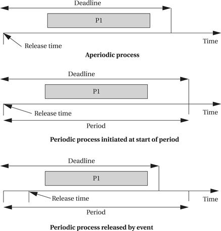
Figure 6.2 Example definitions of initiation times and deadlines.
A deadline specifies when a computation must be finished. The deadline for an aperiodic process is generally measured from the initiation time because that is the only reasonable time reference. The deadline for a periodic process may in general occur at some time other than the end of the period. As we will see in Section 6.5, some scheduling policies make the simplifying assumption that the deadline occurs at the end of the period.
Rate requirements are also fairly common. A rate requirement specifies how quickly processes must be initiated. The period of a process (also called the initiation interval) is the time between successive executions. For example, the period of a digital filter is defined by the time interval between successive input samples. The process’s rate is the inverse of its period. In a multirate system, each process executes at its own distinct rate. The most common case for periodic processes is for the initiation interval to be equal to the period. However, pipelined execution of processes allows the initiation interval to be less than the period. Figure 6.3 illustrates process execution in a system with four CPUs. The various execution instances of program P1 have been subscripted to distinguish their initiation times. In this case, the initiation interval is equal to one-fourth of the period. It is possible for a process to have an initiation rate less than the period even in single-CPU systems. If the process execution time is significantly less than the period, it may be possible to initiate multiple copies of a program at slightly offset times.
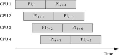
Figure 6.3 A sequence of processes with a high initiation rate.
Jitter
We may also be concerned with the jitter of a task, which is the allowable variation in the completion of the task. Jitter can be important in a variety of applications: in the playback of multimedia data to avoid audio gaps or jerky images; in the control of machines to ensure that the control signal is applied at the right time.
Missing a deadline
What happens when a process misses a deadline? The practical effects of a timing violation depend on the application—the results can be catastrophic in an automotive control system, whereas a missed deadline in a telephone system may cause a temporary silence on the line. The system can be designed to take a variety of actions when a deadline is missed. Safety-critical systems may try to take compensatory measures such as approximating data or switching into a special safety mode. Systems for which safety is not as important may take simple measures to avoid propagating bad data, such as inserting silence in a phone line, or may completely ignore the failure.
Even if the modules are functionally correct, their timing behavior can introduce major execution errors. Application Example 6.2 describes a timing problem in space shuttle software that caused the delay of the first launch of the shuttle.
Application example 6.2 A Space Shuttle Software Error
Garman [Gar81] describes a software problem that delayed the first launch of the U.S. space shuttle. No one was hurt and the launch proceeded after the computers were reset. However, this bug was serious and unanticipated.
The shuttle’s primary control system was known as the Primary Avionics Software System (PASS). It used four computers to monitor events, with the four machines voting to ensure fault tolerance. Four computers allowed one machine to fail while still leaving three operating machines to vote, such that a majority vote would still be possible to determine operating procedures. If at least two machines failed, control was to be turned over to a fifth computer called the Backup Flight Control System (BFS). The BFS used the same computer, requirements, programming language, and compiler, but it was developed by a different organization than the one that built the PASS to ensure that methodological errors did not cause simultaneous failure of both systems. The switchover from PASS to BFS was controlled by the astronauts.
During normal operation, the BFS would listen to the operation of the PASS computers so that it could keep track of the state of the shuttle. However, BFS would stop listening when it thought that PASS was compromising data fetching. This would prevent PASS failures from inadvertently destroying the state of the BFS. PASS used an asynchronous, priority-driven software architecture. If high-priority processes take too much time, the operating system can skip or delay lower-priority processing. The BFS, in contrast, used a time-slot system that allocated a fixed amount of time to each process. Because the BFS monitored the PASS, it could get confused by temporary overloads on the primary system. As a result, the PASS was changed late in the design cycle to make its behavior more amenable to the backup system.
On the morning of the launch attempt, the BFS failed to synchronize itself with the primary system. It saw the events on the PASS system as inconsistent and therefore stopped listening to PASS behavior. It turned out that all PASS and BFS processing had been running late relative to telemetry data. This occurred because the system incorrectly calculated its start time.
After much analysis of system traces and software, it was determined that a few minor changes to the software had caused the problem. First, about two years before the incident, a subroutine used to initialize the data bus was modified. Because this routine was run prior to calculating the start time, it introduced an additional, unnoticed delay into that computation. About a year later, a constant was changed in an attempt to fix that problem. As a result of these changes, there was a 1 in 67 probability for a timing problem. When this occurred, almost all computations on the computers would occur a cycle late, leading to the observed failure. The problems were difficult to detect in testing because they required running through all the initialization code; many tests start with a known configuration to save the time required to run the setup code. The changes to the programs were also not obviously related to the final changes in timing.
The timing constraints between processes may be constrained when the processes pass data among each other. Figure 6.4 shows a set of processes with data dependencies among them. Before a process can become ready, all the processes on which it depends must complete and send their data to it. The data dependencies define a partial ordering on process execution—P1 and P2 can execute in any order (or in interleaved fashion) but must both complete before P3, and P3 must complete before P4. All processes must finish before the end of the period. The data dependencies must form a directed acyclic graph (DAG)—a cycle in the data dependencies is difficult to interpret in a periodically executed system.
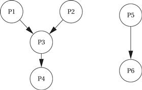
Figure 6.4 Data dependencies among processes.
A set of processes with data dependencies is known as a task graph. Although the terminology for elements of a task graph varies from author to author, we will consider a component of the task graph (a set of nodes connected by data dependencies) as a task and the complete graph as the task set.
Communication among processes that run at different rates cannot be represented by data dependencies because there is no one-to-one relationship between data coming out of the source process and going into the destination process. Nevertheless, communication among processes of different rates is very common. Figure 6.5 illustrates the communication required among three elements of an MPEG audio/video decoder. Data come into the decoder in the system format, which multiplexes audio and video data. The system decoder process demultiplexes the audio and video data and distributes it to the appropriate processes. Multirate communication is necessarily one way—for example, the system process writes data to the video process, but a separate communication mechanism must be provided for communication from the video process back to the system process.
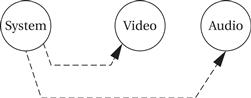
Figure 6.5 Communication among processes at different rates.
6.3.2 CPU Usage Metrics
In addition to the application characteristics, we need to have a basic measure of the efficiency with which we use the CPU. The simplest and most direct measure is utilization:
![]() (Eq. 6.1)
(Eq. 6.1)
Utilization is the ratio of the CPU time that is being used for useful computations to the total available CPU time. This ratio ranges between 0 and 1, with 1 meaning that all of the available CPU time is being used for system purposes. Utilization is often expressed as a percentage.
6.3.3 Process State and Scheduling
The first job of the operating system is to determine the process that runs next. The work of choosing the order of running processes is known as scheduling.
The operating system considers a process to be in one of three basic scheduling states: waiting, ready, or executing. There is at most one process executing on the CPU at any time. (If there is no useful work to be done, an idling process may be used to perform a null operation.) Any process that could execute is in the ready state; the operating system chooses among the ready processes to select the next executing process. A process may not, however, always be ready to run. For instance, a process may be waiting for data from an I/O device or another process, or it may be set to run from a timer that has not yet expired. Such processes are in the waiting state. Figure 6.6 shows the possible transitions between states available to a process. A process goes into the waiting state when it needs data that it has not yet received or when it has finished all its work for the current period. A process goes into the ready state when it receives its required data and when it enters a new period. A process can go into the executing state only when it has all its data, is ready to run, and the scheduler selects the process as the next process to run.
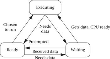
Figure 6.6 Scheduling states of a process.
A scheduling policy defines how processes are selected for promotion from the ready state to the running state. Every multitasking operating system implements some type of scheduling policy. Choosing the right scheduling policy not only ensures that the system will meet all its timing requirements, but it also has a profound influence on the CPU horsepower required to implement the system’s functionality.
Scheduling policies vary widely in the generality of the timing requirements they can handle and the efficiency with which they use the CPU. Utilization is one of the key metrics in evaluating a scheduling policy. We will see that some types of timing requirements for a set of processes imply that we cannot utilize 100% of the CPU’s execution time on useful work, even ignoring context switching overhead. However, some scheduling policies can deliver higher CPU utilizations than others, even for the same timing requirements. The best policy depends on the required timing characteristics of the processes being scheduled.
In addition to utilization, we must also consider scheduling overhead—the execution time required to choose the next execution process, which is incurred in addition to any context switching overhead. In general, the more sophisticated the scheduling policy, the more CPU time it takes during system operation to implement it. Moreover, we generally achieve higher theoretical CPU utilization by applying more complex scheduling policies with higher overheads. The final decision on a scheduling policy must take into account both theoretical utilization and practical scheduling overhead.
6.3.4 Running Periodic Processes
We need to find a programming technique that allows us to run periodic processes, ideally at different rates. For the moment, let’s think of a process as a subroutine; we will call them p1(), p2(), etc. for simplicity. Our goal is to run these subroutines at rates determined by the system designer.
First step: while loop
Here is a very simple program that runs our process subroutines repeatedly:
while (TRUE) {
p1();
p2();
}
This program has several problems. First, it doesn’t control the rate at which the processes execute—the loop runs as quickly as possible, starting a new iteration as soon as the previous iteration has finished. Second, all the processes run at the same rate.
A timed loop
Before worrying about multiple rates, let’s first make the processes run at a controlled rate. One could imagine controlling the execution rate by carefully designing the code—by determining the execution time of the instructions executed during an iteration, we could pad the loop with useless operations (NOPs) to make the execution time of an iteration equal to the desired period. Although some video games were designed this way in the 1970s, this technique should be avoided. Modern processors make it hard to accurately determine execution time, and even simple processors have nontrivial timing as we saw in Chapter 3. Conditionals anywhere in the program make it even harder to be sure that the loop consumes the same amount of execution time on every iteration. Furthermore, if any part of the program is changed, the entire timing scheme must be re-evaluated.
A timer is a much more reliable way to control execution of the loop. We would probably use the timer to generate periodic interrupts. Let’s assume for the moment that the pall() function is called by the timer’s interrupt handler. Then this code will execute each process once after a timer interrupt:
void pall() {
p1();
p2();
}
But what happens when a process runs too long? The timer’s interrupt will cause the CPU’s interrupt system to mask its interrupts (at least on a reasonable processor), so the interrupt won’t occur until after the pall() routine returns. As a result, the next iteration will start late. This is a serious problem, but we will have to wait for further refinements before we can fix it.
Multiple timers
Our next problem is to execute different processes at different rates. If we have several timers, we can set each timer to a different rate. We could then use a function to collect all the processes that run at that rate:
void pA() {
/* processes that run at rate A */
p1();
p3();
}
void pB() {
/* processes that run at rate B */
p2();
p4();
p5();
}
…
This works, but it does require multiple timers, and we may not have enough timers to support all the rates required by a system.
Timer plus counters
An alternative is to use counters to divide the counter rate. If, for example, process p2() must run at 1/3 the rate of p1(), then we can use this code:
static int p2count = 0; /* use this to remember count across timer interrupts */
void pall() {
p1();
if (p2count >= 2) { /* execute p2() and reset count */
p2();
p2count = 0;
}
else p2count++; /* just update count in this case */
}
This solution allows us to execute processes at rates that are simple multiples of each other. However, when the rates aren’t related by a simple ratio, the counting process becomes more complex and more likely to contain bugs.
The next example illustrates an approach to cooperative multitasking in the PIC16F.
Programming Example 6.1 Cooperative Multitasking in the PIC16F887
We can establish a time base using timer 0. The period of the timer is set to the period for the execution of all the tasks. The flag T0IE enables interrupts for timer 0. When the timer finishes, it causes an interrupt and T0IF is set. The interrupt handler for the timer tells us when the timer has ticked using the global variable timer_flag:
void interrupt timer_handler() {
if (T0IE && T0IF) { /* timer 0 interrupt */
timer_flag = 1; /* tell main that the next time period has started */
T0IF = 0; /* clear timer 0 interrupt flag */
}
The main program first initializes the timer and interrupt system, including setting the desired period for the timer. It then uses a while loop to run the tasks at the start of each period:
main() {
init(); /* initialize system, timer, etc. */
while (1) { /* do forever */
if (timer_flag) { /* now do the tasks */
task1();
task2();
task3();
}
}
}
Why not just put the tasks into the timer handler? We want to ensure that an iteration of the tasks completes. If the tasks we executed in timer_handler() but ran past the period, the timer would interrupt again and stop execution of the previous iteration. The interrupted task may be left in an inconsistent state.