
11.9 PROJECTION OPERATION USING THE LINEAR PROJECTION OPERATOR
In Section 11.8, we discussed how we can associate a time step value to each point in the computation domain ![]() . In this section, we discuss how we can assign a task to each point in the computation domain
. In this section, we discuss how we can assign a task to each point in the computation domain ![]() . This task could later be assigned to a thread for the case of multithreaded software implementation, or the task could be assigned to a PE for the case of hardware systolic implementation. It is a waste of resources (number of processors or number of threads) to associate a unique processor or thread to each point in the computation domain
. This task could later be assigned to a thread for the case of multithreaded software implementation, or the task could be assigned to a PE for the case of hardware systolic implementation. It is a waste of resources (number of processors or number of threads) to associate a unique processor or thread to each point in the computation domain ![]() . The main reason is that each point is active only for one time instant and is idle the rest of the time. The basic idea then is to allocate one processor or thread to several points of
. The main reason is that each point is active only for one time instant and is idle the rest of the time. The basic idea then is to allocate one processor or thread to several points of ![]() . There are basically three ways of doing this:
. There are basically three ways of doing this:
1.
Use linear projection operator matrix P to reduce the dimensions of ![]() to produce a new computation domain
to produce a new computation domain ![]() whose dimensions k < n. Matrix P has dimensions k × n and its rank is k. For our matrix multiplication example,
whose dimensions k < n. Matrix P has dimensions k × n and its rank is k. For our matrix multiplication example, ![]() was 3-D. The linear projection operation would produce a computation domain
was 3-D. The linear projection operation would produce a computation domain ![]() that is 2-D or 1-D.
that is 2-D or 1-D.
2.
Use a nonlinear operator to reduce the size of the computation domain ![]() , but keep its dimension n fixed. For our matrix multiplication example, the size of
, but keep its dimension n fixed. For our matrix multiplication example, the size of ![]() is a I × J × K cube in 3-D space. The nonlinear operator would produce a new 3-D cube,
is a I × J × K cube in 3-D space. The nonlinear operator would produce a new 3-D cube, ![]() , whose size is now I′ × J′ × K′, where I′ < I, J′ < J and K′ < K.
, whose size is now I′ × J′ × K′, where I′ < I, J′ < J and K′ < K.
3. Use both linear and nonlinear operators to reduce both the size and dimension of the computation domain.
We explain here the first approach since it is the one most used to for design space exploration.
A subtle point to be noticed in the projection operation is that it controls the amount of workload assigned to each software thread for a multithreaded implementation or the workload assigned to each PE for a systolic array implementation. Just like affine scheduling, affine projection affords us little control over the workload assigned to a thread or a PE. However, nonlinear projection operations will give us very good control over the workload assigned to each thread or PE.
11.9.1 The Projection Matrix P
We define a linear projection operation for multithreading as the projection matrix P that maps a point in domain ![]() (of dimension n) to point
(of dimension n) to point ![]() in the k-dimensional computational domain
in the k-dimensional computational domain ![]() according to the equation
according to the equation
The following theorem places a value on the rank of the projection matrix in relation to the dimension of the projected domain.
Theorem 11.4
Given the dimension of ![]() is n and the dimension of
is n and the dimension of ![]() is k and rank(P) is r. Then we must have r = k, that is rank(P) = k, if P is to be a valid projection matrix.
is k and rank(P) is r. Then we must have r = k, that is rank(P) = k, if P is to be a valid projection matrix.
Proof:
P has dimension k × n with k < n. The definition of the rank of a matrix indicates that the rank could not exceed the smaller of n or k. Thus we conclude that r ≤ k.
Now assume that the rank of P is smaller than k. If r < k, then we have r linearly independent rows and k − r rows that are a linear combination of the r rows. Thus, the linear equation given by
(11.82)
![]()
is a system of linear equations in k unknowns, and the number of equations is less than the unknowns. Thus, we have an infinity of solutions. This contradicts our assertion that the mapping matrix maps any point in ![]() to a unique point in
to a unique point in ![]() .
.
Therefore, we conclude that we must have the rank of P equal to k; that is, r = k.
Now the projection matrix P maps two points p1 and p2 in ![]() associated with a particular output variable instance v(c) to the point
associated with a particular output variable instance v(c) to the point ![]() . Thus, we can write
. Thus, we can write
(11.83)
![]()
But from Theorem 11.1 and Eq. 11.27, we can write the expression
(11.84)
![]()
where e is a nullvector associated with the output variable. We conclude therefore that the nullvectors of the projection matrix P are also the nullvectors associated with the output variable v. The following theorem relates the rank of the projection matrix to
Theorem 11.5
Assume the dimension of ![]() is n. If output variable v has r orthogonal nullvectors, then the dimension of
is n. If output variable v has r orthogonal nullvectors, then the dimension of ![]() is k = n − r and the rank of the projection matrix P is k.
is k = n − r and the rank of the projection matrix P is k.
Proof:
The nullvectors of P are the r nullvectors. Thus, the rank of P is given by
(11.85)
![]()
But we proved in Theorem 11.4 that the rank of P is equal to k. Thus, we must have
(11.86)
![]()
Based on this theorem, if our variable had only one nullvector, then the dimension of ![]() will be n − 1. If the variable had two nullvectors, then the dimension of
will be n − 1. If the variable had two nullvectors, then the dimension of ![]() would be n − 2, and so on.
would be n − 2, and so on.
11.9.2 The Projection Direction
A projection matrix is required to effect the projection operation described by Eq. 11.81. However, the projection operation is typically defined in terms of a projection direction, or directions, d. Knowing the desired projection directions helps in finding the corresponding projection matrix P.
Definition 11.1
The projection direction is defined such that any two distinct points, p1 and p2, in ![]() will be projected to the same point in
will be projected to the same point in ![]() if it satisfies the relation
if it satisfies the relation
(11.87)
![]()
where α ≠ 0 is some constant. In other words, the vector connecting p1 and p2 is parallel to d.
Theorem 11.6
The projection direction d is in the nullspace of the projection matrix P.
Proof:
From Definition 11.1, we can write
(11.88)
![]()
(11.89)
![]()
Subtracting the above two equations, we get
(11.90)
![]()
11.9.3 Choosing Projection Direction d
One guideline for choosing a projection direction is the presence of extremal ray r in domain ![]() . An extremal ray is a direction vector in
. An extremal ray is a direction vector in ![]() where the domain extends to infinity or a large value of the indices. The projection matrix should have those rays in its nullspace; that is,
where the domain extends to infinity or a large value of the indices. The projection matrix should have those rays in its nullspace; that is,
(11.91)
![]()
This is just a recommendation to ensure that the dimension of the projected domain ![]() is finite. However, the projection directions do not necessarily have to include the extremal ray directions to ensure a valid multiprocessor. Our 3-D matrix multiplication algorithm deals with matrices of finite dimensions. As such, there are no extremal ray directions. However, we impose two requirements on our multiprocessor.
is finite. However, the projection directions do not necessarily have to include the extremal ray directions to ensure a valid multiprocessor. Our 3-D matrix multiplication algorithm deals with matrices of finite dimensions. As such, there are no extremal ray directions. However, we impose two requirements on our multiprocessor.
A valid scheduling function cannot be orthogonal to any of the projection directions, a condition of Eq. 11.61. Therefore, the projection directions impose restrictions on valid scheduling functions or vice versa. For our matrix multiplication algorithm, we obtained a scheduling function in Eq. 11.73 as
(11.92)
![]()
Possible projection directions that are not orthogonal to s are
(11.93)
![]()
(11.94)
![]()
(11.95)
![]()
In the next section, we will show how matrix P is determined once the projection vectors are chosen.
11.9.4 Finding Matrix P Given Projection Direction d
We present here an algorithm to get the projection matrix assuming we know our projection directions. We start first with the simple case when we have chosen only one projection direction d.
Step 1
Choose the projection directions. In our case, we choose only one projection direction with the value
This choice will ensure that all points along the i-axis will map to one point in ![]() .
.
Step 2
Here we determine the basis vectors for ![]() , such that one of the basis vectors is along d and the other two basis vectors are orthogonal to it. In our case, we have three basis vectors:
, such that one of the basis vectors is along d and the other two basis vectors are orthogonal to it. In our case, we have three basis vectors:
(11.98)
![]()
(11.99)
![]()
Equation 11.97 implies that the i-axis will be eliminated after the projection operation since our choice implies that Pb0 = 0.
Step 3
Choose the basis vectors for ![]() . In this case, we have two basis vectors since the dimension of
. In this case, we have two basis vectors since the dimension of ![]() is two. We choose the basis vectors as
is two. We choose the basis vectors as
(11.100)
![]()
(11.101)
![]()
The above two equations imply that the j-axis will map to ![]() and the k-axis will map to
and the k-axis will map to ![]() . These become the
. These become the ![]() - and
- and ![]() -axes for
-axes for ![]() , respectively.
, respectively.
Step 4
Associate each basis vector ![]() with a basis vector b. Based on that, we can write
with a basis vector b. Based on that, we can write
(11.102)
![]()
Step 5
We now have a sufficient number of equations to find all the elements of the 2 × 3 projection matrix P:
(11.103)
![]()
(11.104)
![]()
The first Equation is a set of two equations. The second Equation is a set of 2 × 2 equations. In all, we have a set of 2 × 3 equations in 2 × 3 unknowns, which are the elements of the projection matrix P.
For our case, we can write the above equations in a compact form as
(11.105)
![]()
Explicitly, we can write
(11.106)
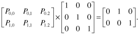
The solution to the above Equation is simple and is given by
Thus, a point ![]() maps to point
maps to point ![]() .
.