Aims

• To demonstrate how spot-rates for different maturities give rise to the (spot) yield curve.
• To show how duration and convexity can be used to provide an approximation to the change in bond prices, after a change in the yield to maturity (YTM).

10.1 YIELD CURVE

Investors borrow (and lend) money over different periods of time. For example, to borrow money today and pay back the principal and interest in 1 year's time, the cost of borrowing might be p.a. To borrow today and pay back the principal and interest in 2 years' time (i.e. there are no interim payments), then the quoted interest rate might be p.a. Because each of these interest rates are quoted for borrowing from today, over a fixed horizon (with no interim payments), they are known as spot-rates (or spot yields).

The (spot) yield curve shows the relationship between (spot) interest rates for different maturity investments. We assume we are dealing with risk-free investments – there is no risk of default. For example, the yield curve at 10 a.m. today might look like that in Figure 10.1. The yield curve in Figure 10.1 is upward sloping, which simply means that if you borrow money at 10 a.m. today then the longer the maturity of your loan, the higher the (spot) interest you will pay. Note that spot-rates apply to a transaction that is conceptually different from a ‘standard loan’. In a standard loan, the repayments schedule will include interim payments and therefore the interest rate charged cannot be called a spot rate.

Spot-rates at any one time are determined in the market by the interplay of the supply of funds by lenders and the demand for funds by borrowers. As the supply and demand for funds changes, then spot-rates will change and the yield curve will alter its shape or position. Usually, if there is a change in demand and supply of funds at a particular horizon (e.g. lending over 2 years) then this will also influence the supply and demand at all other horizons. For example, if increases then all other spot-rates will also tend to increase – the correlation coefficient between changes in any two spot-rates (with different maturities) over a short horizon (e.g. 1 week) is very high, usually in excess of 0.9. Although spot-rates tend to move up and down together, they do not all move by the same absolute amount. In general ‘long-rates’ tend to move less than ‘short-rates’. For example, if the 1-year rate increases by 1% (e.g. from 3% to 4%) over the next week, the 3-year rate might only increase by 0.95% (see curve BB, in Figure 10.1). However, if all spot-rates do happen to move up or down by the same absolute amount this is called a parallel shift in the yield curve.

We have described spot-yields in terms of borrowing and lending money over specific horizons. This can be done by buying a zero-coupon bond (i.e. lending money) or issuing (selling) a ‘zero’ (i.e. borrowing money), so spot-rates can be inferred by observing the market price of zeros. For example, if the market price on a 2-year zero is which pays in 2 years' time then the 2-year spot-rate is 4.26% p.a. (Calculated using . Pure discount government bonds for long maturities do not exist but spot yields can be derived from data on a set of coupon paying bonds (and from swap rates).

Usually the spot-yield curve is upward sloping and flattens out at long maturities. But sometimes it is downward sloping – which implies it costs less to borrow money over say 5 years than it does over one year.

So far we have merely described what the yield curve represents. It tells you how much it will cost you (p.a.) to borrow (or lend) money over a fixed horizon, starting immediately (and with no interim payments). But what determines the shape of the yield curve at any point in time? This analysis is known as the term structure of interest rates and broadly speaking the shape of the yield curve today is determined by the market's expectations about price inflation in future years. If today, inflation is expected to be higher (lower), in each future year then the yield curve will be upward (downward) sloping (see Cuthbertson and Nitzsche 2008).

10.2 DURATION AND CONVEXITY

The duration of a bond is a ‘summary statistic’ which can be used to tell us (approximately) how much the bond price will change, after a change in the yield to maturity (YTM). For example, consider a speculator who currently holds a coupon paying bond with 7 years to maturity, a current market value of $1,000 and which has a duration of . Suppose the YTM moves from 6% to 5.5% over the next week, that is the absolute change in the YTM is . Then the price of the bond will rise by approximately 2.5% over the next week, since it can be shown that:¹

(10.1)

The minus sign in the above formula captures the fact that a fall (rise) in the YTM leads to a rise (fall) in the bond price. Note that the duration formula only gives an approximation to the change in price – the actual (or ‘true’) change in price will differ from that given by the duration formula – but the approximation is quite accurate for small changes in yields (e.g. 25 bps). If we require a more accurate measure of the change in price we need to incorporate a ‘convexity’ adjustment (see below) or use the present value pricing equation (see Chapter 9). The duration formula also assumes that yields at all maturities move by the same (absolute) amount – that is, a parallel shift in the yield curve.

According to the duration formula, the change in value of the bond will be around 2.5% of its current market value of $1,000, that is an increase of $25, so the price of the bond at the end of the week will be close to $1,025. Clearly, duration is useful for fixed-income traders who speculate on changes in interest rates – the larger the duration of the bond, the greater the percentage change in the bond price and hence the greater the (‘market’) risk of the bond.

The relationship between the ‘true’ change in bond price and the change in YTM is shown in Figure 10.2 by the curved or ‘convex’ line. The approximate change in price, given by the duration formula is represented by the ‘tangent line’ (at the current yield of 5%). Any actual price rise will exceed that given by the duration equation – and any actual price fall will be less than that calculated using duration. For small changes in yield, the actual price change and the approximated price change – that given using the duration formula – will be very close because the ‘curve’ and the ‘straight line’ coincide.

10.2.1 Duration of a Portfolio of Bonds

Suppose you hold -bonds. The duration of a portfolio of -bonds is simply a weighted average of the duration of the constituent bonds in the portfolio, where the weights are determined by the market value of the individual bonds:

(10.2)

where (assuming no short-selling) and . For example, if you hold $200m in bonds, each of which has a duration and $400m in bonds each with a duration of , then the duration of the bond portfolio is . This implies that if bond yields change by 1%, the value of your bond portfolio will change by (approximately) 9.33 per cent, hence:

(10.3a)

(10.3b)

where , the change in the YTM, is expressed as a decimal (e.g. if the current YTM is 3% p.a. and falls to 2% p.a. over 1 week then ). For a 1% fall in the YTM over 1 week, the (approximate) change in the (dollar) value of the bond portfolio (over 1 week) is .

It can be shown that the formula for for an -period coupon paying bond (annual payments), where is measured as a ‘compound yield’ (decimal) is:

(10.4)

where the present value of each coupon payment at time , is . In Equation (10.4) the present value of each coupon payment is ‘weighted’ by the ‘time’ at which the coupon is received . Hence, the duration of a bond is sometimes described as a ‘time weighted average term to maturity of the bond’. However, what is important is that today, the duration of any bond can be calculated using (10.4) and an approximate change in the bond price is then given by Equation (10.1) (or Equation (10.5) below).

Duration is a useful summary statistic for calculating (approximate) changes in bond prices but what factors determine the duration of a coupon paying bond? Some useful ‘rules of thumb’ are: (a) duration generally increases with time to maturity (always does so for bonds selling at or above par); (b) duration is higher the lower is the coupon rate (); and (c) duration is (usually) higher when the YTM is low.

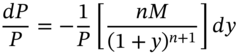
Above we have used the ‘compound yield’ in the duration formula and when this is the case it can be shown (see Appendix 10) that for small changes in (compound) yields, the proportionate change in the bond price is actually given by:

(10.5)

where ‘modified duration’ is defined as . Equation (10.5) is a little more involved than our original formula, Equation (10.1) because of the inclusion of the term in the denominator. Also note that in using this equation we have to express as a proportion – so a yield of 5% would appear in this formula as and an increase in the yield of 1% (over 1 week, say) would imply . If , then the proportionate change in price is , that is, a price fall of 4.76%. (when calculated using compound yields as above) is known as Macaulay duration. Calculation of duration for a coupon bond is illustrated in Example 10.1, along with the approximate price change using the duration formula. Duration provides a good approximation to the change in price of a bond for parallel shifts in the yield curve and for small changes in yields (of up to 25 bp).

Sometimes a useful ‘shorthand’ used by bond traders is to refer to the dollar duration (DD) of a bond which is defined as:

(10.6)

Knowing one can immediately calculate the (approximate) dollar change in value of the bond. Going one step further, for a 1 bp (0.01%) change in the YTM we have , hence:

(10.7)

The expression in (10.7) is known as ‘price value of a basis point’ () or the ‘duration value of a basis point’, usually denoted DV01.

The above equations can be applied to a single bond using that bond's duration or to a portfolio of bonds using the portfolio duration,. For example, to illustrate the use of PVBP, consider a trader who has a portfolio of bonds worth and the portfolio ‘modified duration’ , then PVBP for the portfolio is $500. Suppose there is now a 1 bp change in the yield – for example a change from to – then the change in value of the bond portfolio is .

10.2.2 Convexity

Duration only provides a (first order) approximation to the change in price of a bond and hence is only accurate for small changes in yields (e.g. up to 25 bps). A more accurate approximation is found by incorporating the convexity of the bond. Convexity (with annual coupon payments) is defined as:

(10.8)

Convexity measures the curvature of the price-yield relationship.

Unfortunately, there is really no intuition behind the convexity formula. It arises from the mathematics of approximating the non-linear relationship between the bond price and the YTM, using a second order Taylor series expansion for (see Appendix 10). However, once we have calculated the bond's convexity (in Excel say), our improved estimate for the change in the bond price is given by:

(10.9)

A high value for convexity is a desirable property in a bond since if you can find two bonds with the same duration, then the bond with the highest convexity (i.e. higher curvature in the price-yield relationship) will exhibit a larger rise in price when yields fall and a smaller fall in price when yields rise – compared with the low convexity bond. However, this ‘advantage’ will be reflected in the higher price you have to pay for the ‘high-convexity’ bond.

The price change calculated using duration and ‘duration plus convexity’ are both approximations to the actual ‘true’ price change. The actual (true) price change will differ from that given by (10.9) if either the change in yield is large or there is a non-parallel shift in the yield curve, as shown in Example 10.2.

10.3 SUMMARY

• The spot rate is the rate of interest which applies to money borrowed today and paid back at a single point in the future (with no interim payments).
• The yield curve is a relationship between interest rates for different maturities (taken at a specific time e.g. 10 a.m. Monday, 20 February).
• Duration (or ‘modified duration, ) and convexity can be used to provide an approximation to the change in price (value) of a bond (portfolio), for a given change in the yield to maturity (here assumed to be a compound rate).
  

APPENDIX 10: DURATION AND CONVEXITY

The price of a coupon paying bond, with annual coupon payments is a non-linear (convex) function of the yield to maturity, (compound yield):

(10.A.1)

The change in for any non-linear function can be approximated by a Taylor series expansion:

(10.A.2)

Differentiating (10.A.1) with respect to gives:

(10.A.3)

Using the first term in the Taylor series and (10.A.3) we obtain:

(10.A.4)

Equation (10.A.3) can be written as:

(10.A.5)

where we define duration and ‘modified duration’ as:

(10.A.6a)

(10.A.6b)

Duration and modified duration for a coupon paying bond are calculated using (10.A.6a) and (10.A.6b) where the inputs are the current YTM (for an -period bond), current market price of the bond, the coupons and maturity value of the bond. Having obtained the value for (or ) Equation (10.A.5) provides a first order approximation for the proportionate change in the bond price (for small changes in the YTM and for parallel shifts in the yield curve).

To calculate the change in the bond price using the second order Taylor series expansion (10.A.2) we differentiate (10.A.3) again with respect to :

(10.A.7)

Using (10.A.2), (10.A.4) and (10.A.7) we obtain a second order approximation to the change in the bond price:

(10.A.8)

where we define the ‘convexity’ of the bond as Equation (10.A.7) divided by :

(10.A.9)

The convexity of a coupon paying bond at any point in time can be calculated from (10.A.9). The modified duration and convexity are then used in (10.A.8) to calculate the approximate change in the bond price – over a small interval of time (i.e. is small) – and for a parallel shift in the yield curve.

Zero-coupon Bond

It is straightforward to show that the duration of a zero-coupon bond equals its time to maturity, . We have:

(10.A.10)

(10.A.11)

Substituting for from (10.A.10) in (10.A.11):

(10.A.12)

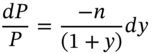
Duration is defined by the following equation:

(10.A.13)

Hence, comparing (10.A.12) and (10.A.13) we see that the duration of a zero-coupon bond equals the time to maturity of the zero. Hence a zero-coupon bond with 5 years (left) to maturity has a duration equal to 5.

Continuously Compounded Yields

Repeating the above analysis using the continuously compounded YTM () to price a coupon paying bond we have:

(10.A.14)

where time of the cash flow in years (e.g. if the coupons are paid 6 months, 1 year, 1.5 years from today, then etc. Using (10.A.14) and a first order Taylor series for , it can be shown that:

(10.A.15)

where duration, using the continuously compounded YTM is defined as:

(10.A.16)

EXERCISES

Question 1

What is the (spot) yield curve and why is it useful?

Question 2

If all yields are expected to fall by 1% over the next week, would you hold low duration or high duration bonds?

Question 3

What is meant by the convexity of a bond? Why might you be willing to pay more for bond-A which has a greater convexity than bond-B (ceteris paribus)?

Question 4

Consider a 5-year, 10% coupon bond (annual coupons) with par value $100, yield to maturity p.a. (compound rate). Calculate the current market price, and the (Macaulay) duration, .

Question 5

Consider a 5-year, 10% coupon bond (annual coupons) with par value $100 and yield to maturity, p.a. (compound rate). The current market price, and the (Macaulay) duration . Calculate:

• 1. The (approximate) price change if the yield to maturity falls to 9.5%.
  2. The ‘true’ price change if falls to 9.5%.

Question 6

• • Portfolio A: 1-year zero-coupon bond, face value = $2,000 and

    10-year zero-coupon bond, face value = $6,000

  • Portfolio B: 5.95-year zero-coupon bond, face value = $5,000

Current yield curve is flat and p.a. (continuously compounded)

• 1. Show that the duration of portfolio-A equals that of portfolio-B.
  2. What is the actual percentage change in value of portfolio-A for an increase in yield of 10 bps?
  3. Does the duration formula give approximately the same answer?
  4. Repeat (b) for portfolios A and B for an increase in yield of 5% p.a. Which portfolio has the higher convexity?