CHAPTER 24
Analysis of Black–Scholes
Aims
- To examine alternative ways of measuring and forecasting volatility.
- To test the validity of the Black–Scholes equation.
- To assess the limitations of the Black–Scholes equation for pricing European options.
24.1 VOLATILITY
In the Black–Scholes formula all variables are directly observable, except for the volatility of stock returns (over the life of the option). To price an option we therefore require a forecast of volatility. Typical values of the annual standard deviation might be in the range of ![]() for individual stocks and around 20% p.a. for stock indices (e.g. S&P 500). If stock returns are assumed to be independent (and identically distributed), the standard deviation over a horizon
for individual stocks and around 20% p.a. for stock indices (e.g. S&P 500). If stock returns are assumed to be independent (and identically distributed), the standard deviation over a horizon ![]() (measured in years or fractions of a year), is given by
(measured in years or fractions of a year), is given by ![]() . For example, if
. For example, if ![]() the standard deviation over 3 months
the standard deviation over 3 months ![]() is
is ![]() . Hence if we use the
. Hence if we use the ![]() -rule (‘root-tee’ rule) we only require a single estimate of
-rule (‘root-tee’ rule) we only require a single estimate of ![]() using returns over some fixed horizon.
using returns over some fixed horizon.
24.1.1 Estimating Volatility
There are a variety of methods used to forecast volatility, including an equally weighted average, an exponentially weighted moving average (EWMA), more complex measures based on high/low ranges for returns, time series models such as ARCH (Autoregressive Conditional Heteroscedasticity) and GARCH (Generalised Autoregressive Conditional Heteroscedasticity), and stochastic volatility models.
24.1.1.1 Equally Weighted
If we have daily observations on the stock price then the daily (continuously compounded) return is:
The mean (daily) return is:
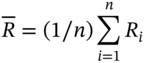
The usual formula for the sample standard deviation is:
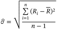
The above formulas can be applied at any chosen frequency for the returns data (e.g. daily, weekly, monthly) to obtain the mean return and standard deviation for any particular horizon.1 For example, using daily returns in (24.3) gives ![]() (i.e. 1% per day) then assuming
(i.e. 1% per day) then assuming ![]() trading days per year, the annual volatility used in the Black–Scholes formula is:
trading days per year, the annual volatility used in the Black–Scholes formula is:
A measure of the accuracy of our estimate of ![]() is given by its standard error (stde). If returns are niid (i.e. normally, independent and identically distributed) then it can be shown that
is given by its standard error (stde). If returns are niid (i.e. normally, independent and identically distributed) then it can be shown that ![]() and if we use
and if we use ![]() daily observations to estimate the standard deviation of
daily observations to estimate the standard deviation of ![]() , then:
, then:
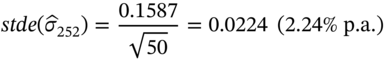
Using only 25 observations means that our estimates of ![]() is not terribly precise. In practice between 90 and 180 days of data are used, thus reducing the standard error to 1.167% or 1.183% p.a. respectively. If the stock pays dividends
is not terribly precise. In practice between 90 and 180 days of data are used, thus reducing the standard error to 1.167% or 1.183% p.a. respectively. If the stock pays dividends ![]() then for those periods which include an ex-dividend day, the continuously compounded stock return is2:
then for those periods which include an ex-dividend day, the continuously compounded stock return is2:
Above, we calculated the annual volatility based on the number of trading days (252) rather than the number of calendar days (365). Which one is ‘correct’ depends on what are the causes of volatility. According to the efficient markets hypothesis (EMH), volatility is caused solely by the random arrival of new information, therefore the volatility over 2 days should be twice that for 1 day. An alternative view is that volatility is caused by the activity of trading itself. French (1980) tested these alternatives. He calculated:
- the variance of daily stock price changes (closing prices) over consecutive trading days (i.e. all closing prices on working days Monday–Friday, if there are no weekday holidays).
- the variance of stock price changes between close of trading on Friday and close of trading on Monday (i.e. 3 calendar days).
If trading and non-trading days are equivalent then the variance in (ii) should equal 3 times the variance in (i). However, French found that results in (ii) are only about 20% higher – hence volatility is far higher when the exchange is open than when it is closed. Proponents of the EMH can of course argue that more information is likely to arise when the exchange is open. But ‘news’ about the weather, which affects agricultural futures prices is equally likely to arise Monday–Friday as on Saturday or Sunday. Hence agricultural futures prices which depend crucially on the weather should obey the ‘3 times’ rule, but they do not (see French and Roll 1986), suggesting it is trading per se that causes volatility. The above arguments suggest that when scaling up daily volatility to an annual volatility we should use ![]() , the number of trading days in a year.
, the number of trading days in a year.
Another question when measuring ![]() is how many past data points to use. If the volatility of stock returns changes dramatically over short time horizons then this suggests using only recent observations to calculate
is how many past data points to use. If the volatility of stock returns changes dramatically over short time horizons then this suggests using only recent observations to calculate ![]() (e.g. the past 90 trading days), since recent data probably more accurately represent the expected volatility over the life of the option contract. On the other hand, using more data points might give a more accurate measure of the ‘true’ volatility, if the latter doesn't vary too much. Some compromise must be reached depending on how time varying the ‘true variance’ is thought to be and there are ‘backtesting’ techniques which can be used to assess the forecasting accuracy of alternative estimates of volatility. A reasonable compromise, for input to the Black–Scholes option pricing equations, might be to estimate
(e.g. the past 90 trading days), since recent data probably more accurately represent the expected volatility over the life of the option contract. On the other hand, using more data points might give a more accurate measure of the ‘true’ volatility, if the latter doesn't vary too much. Some compromise must be reached depending on how time varying the ‘true variance’ is thought to be and there are ‘backtesting’ techniques which can be used to assess the forecasting accuracy of alternative estimates of volatility. A reasonable compromise, for input to the Black–Scholes option pricing equations, might be to estimate ![]() using data over the most recent 90 to 180 trading days.
using data over the most recent 90 to 180 trading days.
There is an inconsistency in using our estimate of ![]() in the Black–Scholes formula since the latter assumes volatility is constant, whereas our historical measure of volatility uses a fixed ‘window’ of n-data points, implying that volatility varies over time (which in practice, it does). However, assuming volatility is constant over the life of the option does not in general lead to large pricing errors.
in the Black–Scholes formula since the latter assumes volatility is constant, whereas our historical measure of volatility uses a fixed ‘window’ of n-data points, implying that volatility varies over time (which in practice, it does). However, assuming volatility is constant over the life of the option does not in general lead to large pricing errors.
24.1.1.2 Exponentially Weighted Moving Average (EWMA)
In the EWMA method, more recent data is given greater weight in forecasting tomorrow's volatility than more distant data. The weights used to forecast volatility are geometrically declining![]() so if
so if ![]() the values of
the values of ![]() are 0.9, 0.81, 0.73, etc. The EWMA volatility forecast is then:
are 0.9, 0.81, 0.73, etc. The EWMA volatility forecast is then:
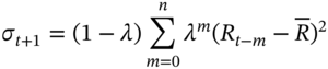
If the sum in Equation (24.7) goes to infinity ![]() , then
, then 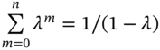 and the weights on past returns sum to unity and the EWMA formula can be rewritten in recursive form:
This simplifies the forecast of volatility. Given an initial value for ![]() , we can ‘update’ each value of
, we can ‘update’ each value of ![]() , namely
, namely ![]() ,
, ![]() ,
, ![]() , …, etc. and the only new piece of information required is
, …, etc. and the only new piece of information required is ![]() for each time period.3 At time t, the forecast one period ahead
for each time period.3 At time t, the forecast one period ahead ![]() , then only requires our previously calculated
, then only requires our previously calculated ![]() and the current value for
and the current value for ![]() – that is, two data points (and not the infinite sum of data points in (24.7)). For forecasting daily volatility we usually assume a zero mean return, hence:
– that is, two data points (and not the infinite sum of data points in (24.7)). For forecasting daily volatility we usually assume a zero mean return, hence:
A ‘best estimate’ of ![]() can be obtained by choosing that value for
can be obtained by choosing that value for ![]() that minimises the ex-post forecast errors of volatility over some past ‘backtesting’ data period. For daily returns
that minimises the ex-post forecast errors of volatility over some past ‘backtesting’ data period. For daily returns ![]() is usually around 0.95.
is usually around 0.95.
24.1.1.3 ARCH and GARCH
More sophisticated methods of forecasting ![]() include ARCH and GARCH regressions. These models assume that the forecast of tomorrow's volatility is a weighted average of today's volatility, plus a ‘surprise’ (or unexpected) contribution due to today's observed stock return. The simple GARCH model is rather similar to the EWMA model and both are autoregressive (i.e. tomorrow's forecast of volatility depends on a weighted average of past volatilities – Cuthbertson and Nitzsche 2004). The GARCH approach is a type of stochastic volatility model, since volatility is partly influenced by past random events.
include ARCH and GARCH regressions. These models assume that the forecast of tomorrow's volatility is a weighted average of today's volatility, plus a ‘surprise’ (or unexpected) contribution due to today's observed stock return. The simple GARCH model is rather similar to the EWMA model and both are autoregressive (i.e. tomorrow's forecast of volatility depends on a weighted average of past volatilities – Cuthbertson and Nitzsche 2004). The GARCH approach is a type of stochastic volatility model, since volatility is partly influenced by past random events.
Consider a simple GARCH model. Daily returns ![]() are assumed to be (conditionally) normally distributed with a mean
are assumed to be (conditionally) normally distributed with a mean ![]() and a time-varying variance,
and a time-varying variance, ![]() :
:
The (conditional) variance of ![]() is time varying,
is time varying, ![]() . The GARCH(1,1) model assumes that volatility is autocorrelated (i.e. tomorrow's variance depends on today's variance).
. The GARCH(1,1) model assumes that volatility is autocorrelated (i.e. tomorrow's variance depends on today's variance).
If ![]() is close to unity then the variance is persistent – periods of high (low) variance or ‘turbulence’ are generally followed by further periods of high (low) variance. GARCH models can utilise any appropriate distribution for the error term and hence are very flexible (e.g. Student's t-distribution, which has fatter tails than the normal distribution). An estimated GARCH equation for daily returns (e.g. on a stock index) might be:
is close to unity then the variance is persistent – periods of high (low) variance or ‘turbulence’ are generally followed by further periods of high (low) variance. GARCH models can utilise any appropriate distribution for the error term and hence are very flexible (e.g. Student's t-distribution, which has fatter tails than the normal distribution). An estimated GARCH equation for daily returns (e.g. on a stock index) might be:
Persistence in variance is indicated by ![]() , which is very close to unity. This means that if volatility
, which is very close to unity. This means that if volatility ![]() is high (low) today it will tend to remain high (low) for a considerable time in the future. The long-run steady state variance is
is high (low) today it will tend to remain high (low) for a considerable time in the future. The long-run steady state variance is ![]() , which implies
, which implies ![]() (1% per day). So the GARCH models implies that day-by-day the standard deviation of stock returns moves in long swings around its long-run mean value of 1% per day, but takes some considerable time to return to its long-run level.
(1% per day). So the GARCH models implies that day-by-day the standard deviation of stock returns moves in long swings around its long-run mean value of 1% per day, but takes some considerable time to return to its long-run level.
Forecasts of volatility (over the life of the option) from the above statistical models can be used as an input for ![]() in the Black–Scholes equation to price option-A (say). But in most cases implied volatilities can be calculated from ‘similar’ options-B (e.g. same or similar underlying asset, same strike but slightly different times to maturity) and these implied volatilities are often used as inputs in the Black–Scholes equation to price option-A, rather than statistical forecasts from ARCH and GARCH models. However, the above statistical forecasting models for volatility are used in value at risk (VaR) calculations, which are discussed in Chapters 44–46.
in the Black–Scholes equation to price option-A (say). But in most cases implied volatilities can be calculated from ‘similar’ options-B (e.g. same or similar underlying asset, same strike but slightly different times to maturity) and these implied volatilities are often used as inputs in the Black–Scholes equation to price option-A, rather than statistical forecasts from ARCH and GARCH models. However, the above statistical forecasting models for volatility are used in value at risk (VaR) calculations, which are discussed in Chapters 44–46.
On a slightly different point, Chiras and Manaster (1978) have examined whether volatility estimates based on historical data (e.g. sample standard deviation using the last 90-day returns), predict future volatility better than do (weighted) implied volatilities. They find that implied volatilities forecast future volatility better than ‘historical volatility’ estimates, implying that option traders are using more information than contained in simple averages of historical data.
24.2 TESTING BLACK–SCHOLES
Tests of the validity of the Black–Scholes equation are joint tests of:
- the assumptions behind the Black–Scholes European option pricing formula are correct
- the market is efficient so that quoted options prices move quickly to equal their no-arbitrage ‘fair value’ given by the Black–Scholes equation.
The Black–Scholes model does not price American options (where early exercise is possible). Hence we only deal with European options. In principle, testing Black–Scholes is very simple. Using current data on the known variables ![]() and a forecast for
and a forecast for ![]() , one can calculate the Black–Scholes theoretical or fair price
, one can calculate the Black–Scholes theoretical or fair price ![]() of a European call (on a non-dividend paying stock). If the actual quoted price of the call option is
of a European call (on a non-dividend paying stock). If the actual quoted price of the call option is ![]() then we expect
then we expect ![]() . In practice, the following difficulties arise in testing the Black–Scholes model:
. In practice, the following difficulties arise in testing the Black–Scholes model:
- Quoted option price
 and the inputs to Black–Scholes, the stock price
  and interest rate
  must be observed synchronously.
 - The estimate of
 used to calculate the Black–Scholes value
  can be calculated in various ways (as discussed above) and each will give a different value for
  .
. - For options on stocks that pay dividends some assumptions have to be made about the timing of future dividend payments.
Market prices for ![]() and
and ![]() might be misleading if they refer to trades separated by even one minute. Since we are dealing with potentially risk-free arbitrage profits, we need ‘high quality’ synchronous data. Similar arguments apply to the choice of the risk-free rate (e.g. should you use the rate on T-bills or the repo rate).
might be misleading if they refer to trades separated by even one minute. Since we are dealing with potentially risk-free arbitrage profits, we need ‘high quality’ synchronous data. Similar arguments apply to the choice of the risk-free rate (e.g. should you use the rate on T-bills or the repo rate).
It is generally found in empirical studies that for at-the-money options ![]() is close to the quoted price
is close to the quoted price ![]() , and the Black–Scholes formula holds. However, for in-the-money (ITM) or out-of-the-money (OTM) options,
, and the Black–Scholes formula holds. However, for in-the-money (ITM) or out-of-the-money (OTM) options, ![]() and the Black–Scholes formula is ‘biased’. But how inaccurate is the Black–Scholes equation? What is important is whether it is possible to make risk-free profits, after taking account of transactions costs (bid–ask spreads) when delta hedging an options portfolio, while waiting for any mispricing to be corrected. The vast amount of evidence on this question suggests that there are very few occasions where even small arbitrage profits can be made (Black and Scholes 1972; Galai 1977) – hence for plain vanilla European options on stocks, stock indices and currencies, the Black–Scholes formula works relatively well.
and the Black–Scholes formula is ‘biased’. But how inaccurate is the Black–Scholes equation? What is important is whether it is possible to make risk-free profits, after taking account of transactions costs (bid–ask spreads) when delta hedging an options portfolio, while waiting for any mispricing to be corrected. The vast amount of evidence on this question suggests that there are very few occasions where even small arbitrage profits can be made (Black and Scholes 1972; Galai 1977) – hence for plain vanilla European options on stocks, stock indices and currencies, the Black–Scholes formula works relatively well.
24.2.1 Implied Volatility
An indirect method of showing that the Black–Scholes formula yields biases is to look at implied volatilities for European call and put options on the same underlying asset (e.g. stocks, foreign currency). If the Black–Scholes equation correctly prices all these options, then their implied volatilities should not vary with the strike price (or time to maturity). For foreign currency options (e.g. on USD/GBP) if we take quoted prices of calls and puts with different strikes (but the same maturity) and back out the implied volatilities (see Chapter 16) we find that a plot of ![]() against
against ![]() produces a ‘smile’ (Figure 24.1).
produces a ‘smile’ (Figure 24.1).
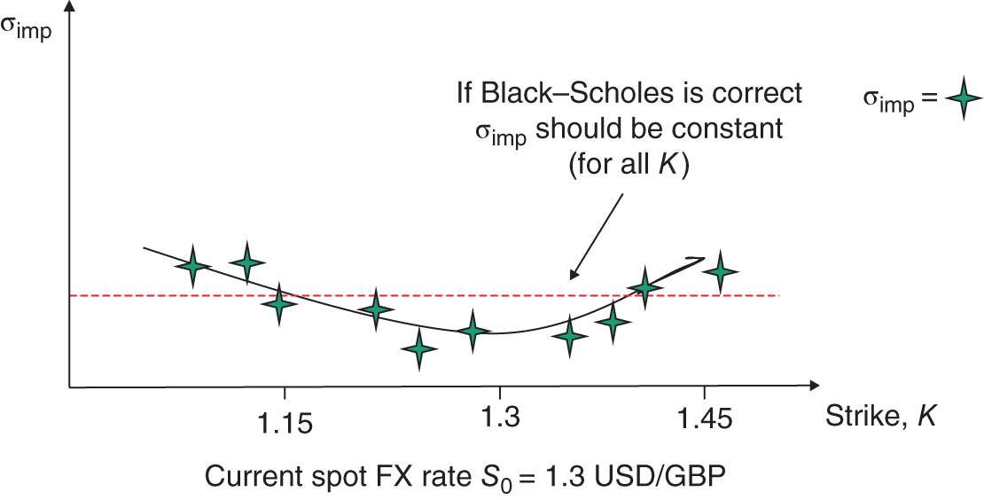
FIGURE 24.1 Volatility smile: USD/GBP
For options on equity indices (e.g. S&P 500) implied volatilities plotted against different strikes produce a volatility skew; implied volatilities for very ‘low’ strikes (e.g. OTM puts) have much higher values of ![]() , than for ATM or ITM puts (Figure 24.2). The above results, qualitatively, also apply to American calls and puts.
, than for ATM or ITM puts (Figure 24.2). The above results, qualitatively, also apply to American calls and puts.
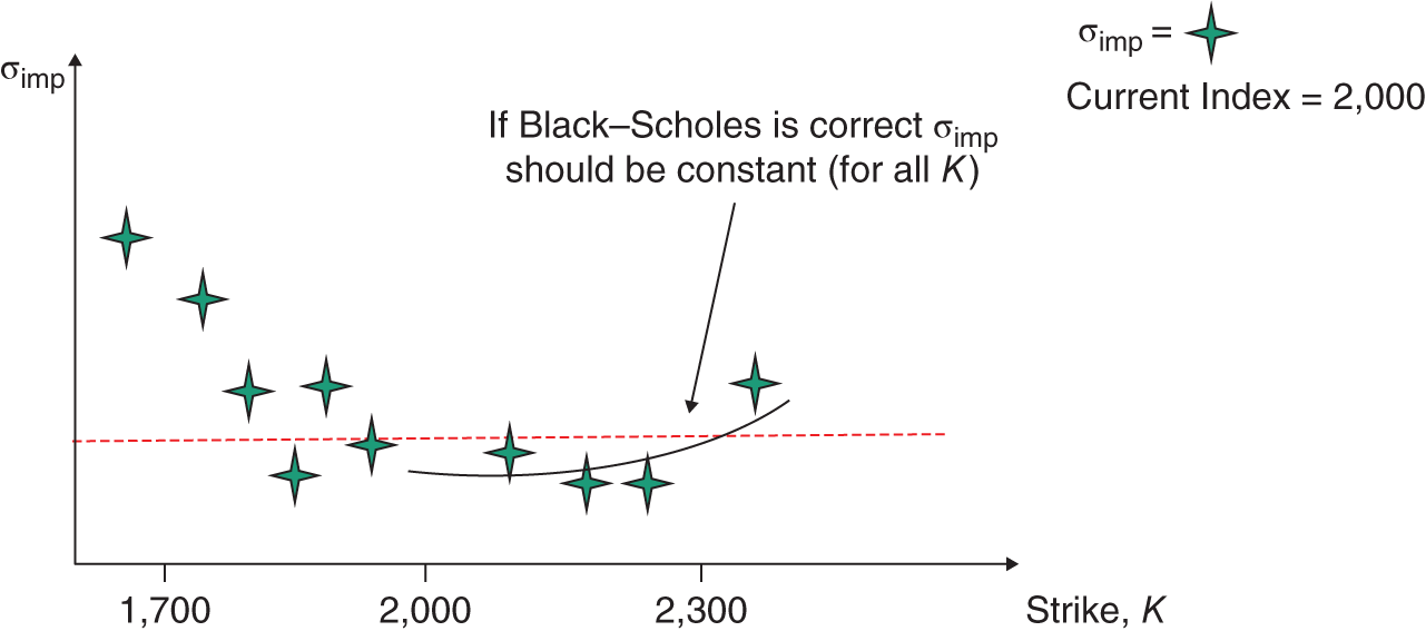
FIGURE 24.2 Volatility skew: equity index
The positions of the graphs in Figures 24.1 and 24.2 depend on the current price of the underlying asset. For example, the lowest point of the volatility smile (Figure 24.1) is usually close to the current spot FX rate and if the spot rate increases (say), the ‘smile curve’ moves to the right. Hence the volatility smile (or skew) is often a plot of ![]() against either
against either ![]() or
or ![]() where
where ![]() is the forward/futures price with maturity
is the forward/futures price with maturity ![]() , the same as the maturity of the options.
, the same as the maturity of the options.
Implied volatilities can also be calculated for calls and puts with different maturities (but on the same underlying and same strike) – this is the term structure of (implied) volatility. Historical implied volatilities for different strikes and maturities are shown in Table 24.1 – this represents the volatility surface. In Table 24.1 for short-dated options (1-month), there is a pronounced volatility smile with respect to the strike price but this becomes less pronounced at longer maturities (e.g. for 5-year maturities).
TABLE 24.1 Volatility surface (% p.a.)
| Time to maturity |
|
|
|
| 1 month | 17.2 | 15.0 | 17.5 |
| 6 months | 17.1 | 15.1 | 17.3 |
| 1 year | 17.6 | 16.5 | 17.8 |
| 5 years | 17.7 | 17.8 | 18.0 |
Some of the values for implied volatilities are obtained directly from prices of liquid options and some values in Table 24.1 will be interpolated. When using implied volatilities to price a ‘new’ call (or put) option-X (on FX say), a financial engineer will look at option-X's current value for ![]() (say) and maturity
(say) and maturity ![]() year (say) and then read off the appropriate value of implied volatility
year (say) and then read off the appropriate value of implied volatility ![]() (Table 24.1). This volatility would be used to price option-X using the Black–Scholes formula or in the BOPM (to calculate U and D) or in a MCS to generate the underlying asset price (see Chapter 26). If option-X has values of
(Table 24.1). This volatility would be used to price option-X using the Black–Scholes formula or in the BOPM (to calculate U and D) or in a MCS to generate the underlying asset price (see Chapter 26). If option-X has values of ![]() or
or ![]() that do not exactly match those in Table 24.1 then interpolation is used.
that do not exactly match those in Table 24.1 then interpolation is used.
Volatility is found to be mean reverting, so if short-term volatility is below (above) its long-run level then it tends to increase (decrease) over longer horizons. Hence, when short-term volatility is historically low, implied volatility tends to be an increasing function of maturity – as in the columns of Table 24.1. (The opposite is true when historical volatility is high.)
Some practitioners define the volatility smile as the relationship between ![]() and
and ![]() and then ‘the smile’ is less dependent on T. With enough data points in Table 24.1 it may be possible to run a regression of
and then ‘the smile’ is less dependent on T. With enough data points in Table 24.1 it may be possible to run a regression of ![]() against
against ![]() and (some function of)
and (some function of) ![]() to give
to give ![]() . Given the estimated values of
. Given the estimated values of ![]() you can then directly calculate the value for
you can then directly calculate the value for ![]() for option-X.
for option-X.
24.3 LIMITATIONS OF BLACK–SCHOLES
Using the Black–Scholes formula only gives the ‘correct’ (no-arbitrage) price if the assumptions underlying the mathematical model are true and if the market eliminates all (risk-free) arbitrage opportunities. Empirical studies show that the Black–Scholes formula does accurately price ATM options but not ITM or OTM options. A key assumption of the Black–Scholes model is that the continuously compounded stock return is ![]() , which implies that the stock price (at maturity of the option contract) is lognormal. Not surprisingly, if the ‘true’ (empirical) distribution of the stock price is not lognormal, then the quoted price will differ from the Black–Scholes price.
, which implies that the stock price (at maturity of the option contract) is lognormal. Not surprisingly, if the ‘true’ (empirical) distribution of the stock price is not lognormal, then the quoted price will differ from the Black–Scholes price.
For example, a significantly OTM call option has a positive value only if there is a large increase in the stock price (so that at expiration ![]() ), where the right tail of the stock price distribution matters. The fatter the right tail of the terminal stock price distribution, the more valuable the call option. Hence, if the true distribution for the stock price has a right tail which is ‘fatter’ than the lognormal distribution, the Black–Scholes formula will tend to underprice this option (relative to the market's correct valuation based on the true fat tailed distribution). A similar argument can be made if the right tail is thinner than the lognormal. Here the traded price of the call will be below that given by the Black–Scholes formula.
), where the right tail of the stock price distribution matters. The fatter the right tail of the terminal stock price distribution, the more valuable the call option. Hence, if the true distribution for the stock price has a right tail which is ‘fatter’ than the lognormal distribution, the Black–Scholes formula will tend to underprice this option (relative to the market's correct valuation based on the true fat tailed distribution). A similar argument can be made if the right tail is thinner than the lognormal. Here the traded price of the call will be below that given by the Black–Scholes formula.
For an out-of-the-money put, a positive payoff at maturity requires a fall in stock prices, hence if the true terminal distribution for the stock price has a fatter left tail than the lognormal, then the Black–Scholes formula will underprice the OTM put.
The Black–Scholes model assumes a constant volatility, which must be independent of the stock price. However, suppose the stock price is positively correlated with volatility. This implies that when ![]() is high, the right tail of the distribution will be ‘fat’ and the left tail ‘thin’ (relative to the constant volatility case). Hence the Black–Scholes formula will misprice ITM and OTM options. These distortions in the Black–Scholes price are due to the assumption of a constant volatility and will increase with the time to maturity of the option (because
is high, the right tail of the distribution will be ‘fat’ and the left tail ‘thin’ (relative to the constant volatility case). Hence the Black–Scholes formula will misprice ITM and OTM options. These distortions in the Black–Scholes price are due to the assumption of a constant volatility and will increase with the time to maturity of the option (because ![]() and hence any mismeasurement of
and hence any mismeasurement of ![]() is magnified as
is magnified as ![]() increases).
increases).
24.3.1 Jump Diffusion Process
The Black–Scholes formula assumes ![]() is
is ![]() . However, if the true distribution is one where from time-to-time relatively large positive or negative ‘jumps’ occur then the true distribution has ‘fat’ right and left tails and the Black–Scholes formula will misprice the options. We explore some implications of the stock price being subject to ‘jumps’. A geometric Brownian motion for the stock price:
. However, if the true distribution is one where from time-to-time relatively large positive or negative ‘jumps’ occur then the true distribution has ‘fat’ right and left tails and the Black–Scholes formula will misprice the options. We explore some implications of the stock price being subject to ‘jumps’. A geometric Brownian motion for the stock price:
gives a lognormal distribution for the terminal stock price. The stock price is equally likely to increase or decrease because ![]() . Suppose we want to generate a series for the stock price that exhibits both larger and more frequent ‘sharp’ price falls than given by the lognormal distribution. This can be represented by a jump diffusion process. When
. Suppose we want to generate a series for the stock price that exhibits both larger and more frequent ‘sharp’ price falls than given by the lognormal distribution. This can be represented by a jump diffusion process. When ![]() is negative, Equation (24.13) implies that this contributes to a fall in the stock price. We want ‘occasionally’ to make the stock price fall by more than given by Equation (24.13). Let the size of the jump be
is negative, Equation (24.13) implies that this contributes to a fall in the stock price. We want ‘occasionally’ to make the stock price fall by more than given by Equation (24.13). Let the size of the jump be ![]() and the frequency or intensity of the jumps,
and the frequency or intensity of the jumps, ![]() . We simply add the following term to Equation (24.13) (in Excel):
. We simply add the following term to Equation (24.13) (in Excel):
The function ![]() draws any number between 0 and 1 with equal probability. If
draws any number between 0 and 1 with equal probability. If ![]() is less than
is less than ![]() then the ‘IF’ statement takes a value of 1 and the whole expression equals
then the ‘IF’ statement takes a value of 1 and the whole expression equals ![]() , and hence the stock price undergoes an additional fall. For example, if
, and hence the stock price undergoes an additional fall. For example, if ![]() then the stock price falls by an additional 20%. On the other hand, if
then the stock price falls by an additional 20%. On the other hand, if ![]() returns a ‘large’ positive number, then ‘IF’ returns a ‘0’ and the stock price follows the usual niid process of Equation (24.13). The frequency with which the jumps occur is usually taken to follow a Poisson process. Hence, if the jump is denoted
returns a ‘large’ positive number, then ‘IF’ returns a ‘0’ and the stock price follows the usual niid process of Equation (24.13). The frequency with which the jumps occur is usually taken to follow a Poisson process. Hence, if the jump is denoted ![]() then:
then:
There is a probability ![]() of a jump
of a jump ![]() in time period
in time period ![]() . Thus the jump diffusion process introduces a fat left tail (and a ‘left’ skewed distribution). However, in practice, if there are jumps, then traders cannot perfectly delta hedge. Traders can choose to either hedge only the small ‘Brownian motion changes’ given by (24.13) or they can choose the hedge ratio to minimise the variance in the value of their hedge portfolio, which is now subject to the jump process. Neither approach is particularly satisfactory. In the former case traders are not completely hedged when a large fall in the stock price occurs and in the latter case they are only hedged for large changes ‘on average’ – and this may be of little comfort immediately after a substantial crash.
. Thus the jump diffusion process introduces a fat left tail (and a ‘left’ skewed distribution). However, in practice, if there are jumps, then traders cannot perfectly delta hedge. Traders can choose to either hedge only the small ‘Brownian motion changes’ given by (24.13) or they can choose the hedge ratio to minimise the variance in the value of their hedge portfolio, which is now subject to the jump process. Neither approach is particularly satisfactory. In the former case traders are not completely hedged when a large fall in the stock price occurs and in the latter case they are only hedged for large changes ‘on average’ – and this may be of little comfort immediately after a substantial crash.
Turning back to option pricing. Another alternative is to assume an upper and lower range ![]() and
and ![]() for the possible values of the volatility (estimated from the empirical jump process) and price the option based on the ‘worse case’ outcome. Here one makes no assumptions about the probability distribution of the timing (frequency/intensity) of the crash and we do not need to estimate the average size of the fall
for the possible values of the volatility (estimated from the empirical jump process) and price the option based on the ‘worse case’ outcome. Here one makes no assumptions about the probability distribution of the timing (frequency/intensity) of the crash and we do not need to estimate the average size of the fall ![]() or the probability distribution of
or the probability distribution of ![]() . The only assumption needed is to place an upper bound on the size of the fall and to limit the number of crashes per unit of time (e.g. no more than three crashes per year and that immediately after a crash, there cannot be a crash within the next 6 months). This is a considerable simplification and avoids potential estimation error (see Wilmott 1998, who calls this ‘crash modelling’ and also proposes a ‘Platinum Hedge’ to minimise risk).
. The only assumption needed is to place an upper bound on the size of the fall and to limit the number of crashes per unit of time (e.g. no more than three crashes per year and that immediately after a crash, there cannot be a crash within the next 6 months). This is a considerable simplification and avoids potential estimation error (see Wilmott 1998, who calls this ‘crash modelling’ and also proposes a ‘Platinum Hedge’ to minimise risk).
Where the option price depends on the price of more than one underlying asset (e.g. on two different stock prices) then we need to make some additional assumptions about the correlation of these prices in crash periods. For example, we could assume independence (not particularly realistic) or we could assume all assets fall by the same proportionate amount at the same time (slightly more realistic).
With certain types of jump processes it is possible to obtain a partial differential equation (PDE) for the option price, solve this numerically and hence price the option. For example, if the jump component of the asset return represents non-systematic risk (i.e. the risk is not priced) then we can still apply risk-neutral valuation to obtain a (complex) closed-form solution for a European call option (Merton 1976; Naik and Lee 1990). However, this ‘theoretical price’ depends on the estimated parameters ![]() and
and ![]() of the jump process, which are subject to error. Perhaps this is why jump diffusion models are not widely used to price options. The potential advantages are just not worth the effort and traders prefer to stick with the Brownian motion assumption for
of the jump process, which are subject to error. Perhaps this is why jump diffusion models are not widely used to price options. The potential advantages are just not worth the effort and traders prefer to stick with the Brownian motion assumption for ![]() and ‘trade with their eyes wide shut’ as far as ‘jumps’ are concerned.
and ‘trade with their eyes wide shut’ as far as ‘jumps’ are concerned.
In Chapter 26 we determine option prices using Monte Carlo simulation and this technique requires a ‘representative’ stock price process. There is nothing to stop us using a jump diffusion process for stock prices and if so, we will obtain a different value for the option premium to that given by the Black–Scholes formula (which assumes a geometric Brownian motion). ‘Jumps’ tend to have a greater effect on option premia when the option is close to maturity. Over longer horizons the jumps tend to ‘average out’. However, Ball and Torous (1985) for standard ‘plain vanilla’ options find no significant differences between the Black–Scholes formula and option premia based on ‘jump processes’. However, this conclusion would not hold for certain exotic options (e.g. barrier options).
Intuitively, to see how a very specific ‘jump process’ can influence the call premium, take a simple yet extreme example. It may be that a special event, such as the threat of a takeover, is imminent. In this case traders may anticipate a very large jump depending on the outcome of the takeover – a price rise if the takeover is successful and a price fall if it is not. This probability distribution is bimodal around the expected ‘high’ or ‘low’ price. Therefore the Black–Scholes formula does not apply here and observed option premia on such stocks should differ from those given by Black–Scholes.
24.4 SUMMARY
- In the Black–Scholes formula, option premia are very sensitive to the input for volatility. Forecasts of volatility can be obtained from the sample variance, from exponentially weighted forecasts and from more sophisticated statistical models such as ARCH/GARCH.
- Most options are priced by ‘backing out’ a value for implied volatility from an option-B which is ‘similar’ to ‘option-A’ you wish to price (e.g. option-B would be on the same underlying asset as option-A but would have a different strike price or time to maturity). Several values for implied volatility can be obtained from the prices of traded options-B (e.g. options-B which are ATM, ITM, and OTM). These different implied volatilities from options-B are then used to obtain a ‘best estimate’ for implied volatility (usually a weighted average), which is then used as an input into the Black–Scholes formula to price option-A.
- The Black–Scholes formula exhibits some systematic mispricing patterns, nevertheless it is accurate for pricing a wide range of plain vanilla European options on stocks (which are close to being ATM).
- Stock prices may be subject to large infrequent ‘jumps’. Jump diffusion processes can be incorporated into (some) options pricing models and these models will generally result in different option prices to those given by the Black–Scholes equation.
EXERCISES
Question 1
The volatility of the change in the stock price is 40% p.a. What is the standard deviation of the stock price change over 1 trading day? Assume 252 trading days in a year. What assumptions are you making about the stochastic behaviour of the stock price?
Question 2
The EWMA model can be represented as ![]() with
with ![]() and we assume the mean value for R is zero. Express this equation in terms of the change in the variance (over time)
and we assume the mean value for R is zero. Express this equation in terms of the change in the variance (over time) ![]() and briefly comment on your interpretation of this equation as ‘mean reverting’.
and briefly comment on your interpretation of this equation as ‘mean reverting’.
Question 3
Why do we scale up our estimate of daily volatility to annual values by using trading days rather than calendar days?
Question 4
What, if any, is the intuition behind using the EWMA forecasting scheme for volatility?
The EWMA can be written as either:
- (1)
Which for large n can be shown to be equivalent to:
- (2)
Question 5
A European call option on a stock (with 3 months to maturity) has a quoted price which is 1% below the ‘correct’ (no-arbitrage) Black–Scholes price. How might you take advantage of this mispricing over the next 4 weeks, without incurring a high level of risk?
Question 6
Suppose you calculate implied volatilities from the quoted prices of European calls and puts on the same stock, with the same maturity date, but the options have different strike prices. If the Black–Scholes equation correctly prices these options, what would you expect to observe in a graph of implied volatility (on the y-axis) against the different strike prices (on the x-axis)?
Question 7
The GARCH(1,1) model can be represented as:
- (1)

- (2)

The EWMA model (with an assumption of zero mean return) can be represented as:
- (3)
What assumptions are required, so that the GARCH(1,1) model is equivalent to the EWMA model?
NOTES
- 1 Usually non-overlapping data is used. Using overlapping data creates additional problems. For example, if you use daily returns data to measure the return over 5 days, and then move forward one day at a time, each 5-day return has 4 days in common, so this introduces serial correlation into the 5-day returns series. Non-overlapping data would measure the 5-day return, by moving forward 5 days at a time.
- 2 We have ignored any complications due to the taxation of dividends. If the tax implications are complex then sometimes data that includes an ex-dividend date are excluded from the calculation of
 and hence of
  .
. - 3 If we are using daily data then the initial value for
 is usually taken to be the (standard) sample variance using about 25 daily returns, at the beginning of the data set. Using the recursion in Equation (24.8), the forecast value of
  for about 80 days later is then independent of our (arbitrarily chosen) starting value for
  .
.