
d.c. circuit analysis
Publisher Summary
This chapter focuses on the analysis of direct current (d.c.) circuit. The laws that determine the currents and voltage drops in d.c. networks are (1) Ohm’s law, (2) the laws for resistors in series and in parallel, and (3) Kirchhof’s laws. Kirchhof’s laws consist of two parts, namely, current law and voltage law. Current law states that at any junction in an electric circuit, the total current flowing toward that junction is equal to the total current flowing away from the junction. Voltage law states that in any closed loop in a network, the algebraic sum of the voltage drops, that is products of current and resistance, taken around the loop is equal to the resultant emf acting in that loop. The chapter presents general hints on simple d.c. circuit analysis. There are a number of circuit theorems that have been developed for solving problems in d.c. electrical networks.
Kirchhoff’s laws
At any junction in an electric circuit the total current flowing towards that junction is equal to the total current flowing away from the junction, i.e. ΣI= 0
Thus, referring to Figure 6.1
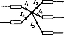
I1 + I2 = I3 + I4 + I5 or I1 + I2 − I3 − I4 − I5 = 0
In any closed loop in a network, the algebraic sum of the voltage drops (i.e. products of current and resistance) taken around the loop is equal to the resultant emf acting in that loop.
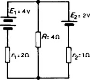
Thus, referring to Figure 6.2:

(Note that if current flows away from the positive terminal of a source, that source is considered by convention to be positive. Thus moving anticlockwise around the loop of Figure 6.2, E1 is positive and E2 is negative.)
For example, using Kirchhoff’s laws to determine the current flowing in each branch of the network shown in Figure 6.3, the procedure is as follows:
(i) Use Kirchhoff’s current law and label current directions on the original circuit diagram. The directions chosen are arbitrary, but it is usual, as a starting point, to assure that current flows from the positive terminals of the batteries. This is shown in Figure 6.4 where the three branch currents are expressed in terms of I1 and I2 only, since the current through R is I1 + I2.
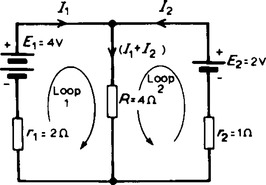
(ii) Divide the circuit into two loops and apply Kirchhoff’s voltage law to each. From loop 1 of Figure 6.4, and moving in a clockwise direction as indicated (the direction chosen does not matter) gives
 (1)
(1)From loop 2 of Figure 6.4, and moving in an anticlockwise direction as indicated (once again, the choice of direction does not matter; it does not have to be in the same direction as that chosen from the first loop), gives:
 (2)
(2)(i.e. I2 is flowing in the opposite direction to that shown in Figure 6.4).
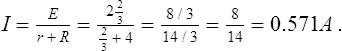
Current flowing through R = I1 + I2 = 0.857 + (− 0.286)=0.571 A.
3. General hints on simple d.c. circuit analysis
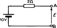
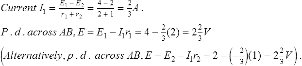
(i) The open-circuit voltage, E, across terminals AB in Figure 6.5 is equal to 10 V, since no current flows through the 2 Ω resistor and hence no voltage drop occurs.
(ii) The open-circuit voltage, E, across terminals AB in Figure 6.6(a) is the same as the voltage across the 6 Ω resistor. The circuit may be redrawn as shown in Figure 6.6(b).

by voltage division in a series circuit.
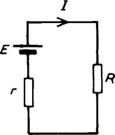
(iii) For the circuit shown in Figure 6.7(a) representing a practical source supplying energy, V = E − Ir where E is the battery emf, V is the battery terminal voltage and r is the internal resistance of the battery. For the circuit shown in Figure 6.7(b),
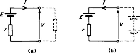
V = E − (− I)r, i.e. V = E + Ir
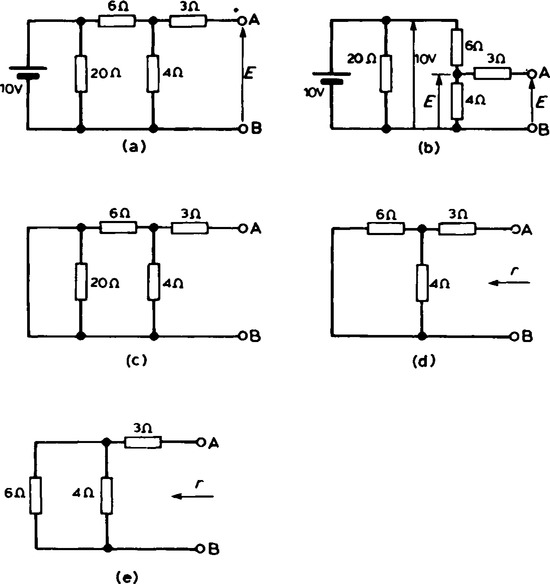
(iv) The resistance ‘looking-in’ at terminals AB in Figure 6.8(a) is obtained by reducing the circuit in stages as shown in Figures 6.8(b) to (d). Hence the equivalent resistance across AB is 7 Ω.

(v) For the circuit shown in Figure 6.9(a), the 3Ω resistor carries no current and the p.d. across the 20Ω resistor is 10 V. Redrawing the circuit gives Figure 6.9(b), from which
(vi) If the 10 V battery in Figure 6.9(a) is removed and replaced by a short-circuit, as shown in Figure 6.9(c), then the 20 Ω resistor may be removed. The reason for this is that a short-circuit has zero resistance, and 20 Ω in parallel with zero ohms gives an equivalent resistance of
The circuit is then as shown in Figure 6.9(d), which is redrawn in Figure 6.9(e). From Figure 6.9(e), the equivalent resistance across AB,
(vii) To find the voltage across AB in Figure 6.10: Since the 20 V supply is across the 5Ω and 15 Ω resistors in series then, by voltage division, the voltage drop across AC,
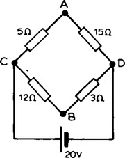
VC is at a potential of + 20 V.
Hence the voltage between AB is
and current would flow from A to B since A has a higher potential than B.
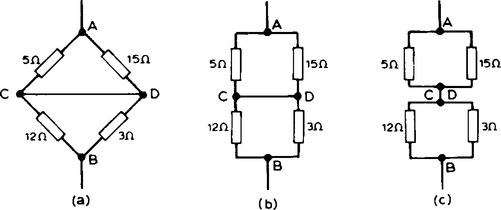
(viii) In Figure 6.11(a), to find the equivalent resistance across AB, the circuit may be redrawn as in Figures 6.11(b) and (c). From Figure 6.11(c), the equivalent resistance across AB
4. There are a number of circuit theorems which have been developed for solving problems in d.c. electrical networks.
5. The superposition theorem states:
‘In any network made up of linear resistances and containing more than one source of emf, the resultant current flowing in any branch is the algebraic sum of the currents that would flow in that branch if each source was considered separately, all other sources being replaced at that time by their respective internal resistances.’
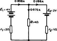
For example, to determine the current in each branch of the network shown in Figure 6.12 using the superposition theorem, the procedure is as follows.

(i) Redraw the original circuit with source E2 removed, being replaced by r2 only, as shown in Figure 6.13(a).

(ii) Label the currents in each branch and their directions as shown in Figure 6.13(a) and determine their values. (Note that the choice of current directions depends on the battery polarity, which, by convention is taken as flowing from the positive battery terminal as shown.) R in parallel with r2 gives an equivalent resistance of
From the equivalent circuit of Figure 6.13(b)
(iii) Redraw the original circuit with source E1 removed, being replaced by r1 only, as shown in Figure 6.14(a)

(iv) Label the currents in each branch and their directions as shown in Figure 6.14(a) and determine their values. r1 in parallel with R gives an equivalent resistance
From the equivalent circuit of Figure 6.14(b):

From Figure 6.14(a)
(v) Superimpose Figure 6.14(a) onto Figure 6.13(a) as shown in Figure 6.15
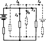
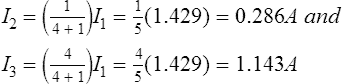
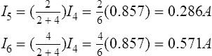
(vi) Determine the algebraic sum of the currents flowing in each branch. Resultant current flowing through source 1, i.e.
Resultant current flowing through source 2, i.e.
Resultant current flowing through resistor R, i.e.
I2 + I5 = 0.286 + 0.286 = 0.572 A.
The resultant currents with their directions are shown in Figure 6.16.
(a) Thévenin’s theorem states:
‘The current in any branch of a network is that which would result if an emf, equal to the p.d. across a break made in the branch, were introduced into the branch, all other emf’s being removed and represented by the internal resistances of the sources.’
(b) The procedure adopted when using Thévenin’s theorem is summarised below. To determine the current in any branch of an active network (i.e. one containing a source of emf):
(i) remove the resistance R from that branch,
(ii) determine the open-circuit voltage, E, across the break,
(iii) remove each source of emf and replace them by their internal resistances and then determine the resistance, r, looking-in’ at the break.
(iv) determine the value of the current from the equivalent circuit shown in Figure 6.17,
For example, using Thévenin’s theorem to determine the current flowing in the 4 Ω resistor shown in Figure 6.18(a)., using the above procedure:

(i) The 4 Ω resistor is removed from the circuit as shown in Figure 6.18(b)
(iii) Removing the sources of emf gives the circuit shown in Figure 6.18(c), from which resistance
(iv) The equivalent Thévenin’s circuit is shown in Figure 6.18(d) from which current
(c) Thévenin’s theorem can be used to analyse part of a circuit, and in complicated networks the principle of replacing the supply by a constant voltage source in series with a resistance is very useful.
‘The current that flows in any branch of a network is the some as that which would flow in the branch if it was connected across a source of electricity, the short-circuit current of which is equal to the current that would flow in a short-circuit across the branch, and the internal resistance of which is equal to the resistance which appears across the open-circuited branch terminals.’
(b) The procedure adopted when using Norton’s theorem is summarised below. To determine the current in any branch AB of an active network:
(i) short-circuit that branch,
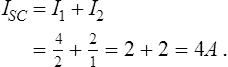
(ii) determine the short-circuit current, ISC,
(iii) remove each source of emf and replace them by their internal resistances (or, if a current source exists replace with an open circuit), then determine the resistance, R, “looking-in” at a break made between A and B,
(iv) determine the value of the current from the equivalent circuit shown in Figure 6.19,

For example, to determine the current flowing in the 4 Ω resistor of Figure 6.18(a) using Norton’s theorem by the above procedure:
(i) the branch containing the 4 Ω resistor is short-circuited as shown in Figure 6.20(a).

(ii) the short-circuit current ISC is given by:
(iii) resistance R = ![]() Ω (same as procedure (iii) of para. 6)
Ω (same as procedure (iii) of para. 6)
(iv) from the equivalent Norton circuit shown in Figure 6.21


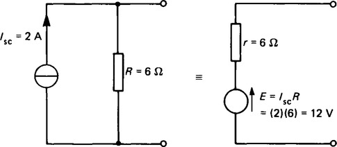
8. Thévénin equivalent circuit having emf E and internal resistance r can be replaced by a Norton equivalent circuit containing a current generator ISC and internal resistance R, where:

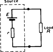
(a) The maximum power transfer theorem states:
‘The power transferred from a supply source to a load is at its maximum when the resistance of the load is equal to the internal resistance of the source.’
Hence, in Figure 6.24, when R = r the power transferred from the source to the load is a maximum.
(b) (b) Varying a load resistance to be equal, or almost equal, to the source internal resistance is called resistance matching. Examples where resistance matching is important include coupling an aerial to a transmitter or receiver, or in coupling a loudspeaker to an amplifier where coupling transformers may be used to give maximum power transfer (see chapter 20, para 11, page 176).
With d.c. generators or secondary cells, the internal resistance is usually very small. In such cases, if an attempt is made to make the load resistance as small as the source internal resistance, overloading of the source results.