
d.c. transients
Publisher Summary
This chapter discusses the direct current (d.c.) transients. When a direct current (d.c.) voltage is applied to a capacitor C, and resistor R connected in series, there is a short period of time immediately after the voltage is connected, during which the current flowing in the circuit and the voltages across C and R are changing. These changing values are called transients. There are two main methods of drawing transient curves graphically, namely, the tangent method and the initial slope and three point method. For a growth curve, the value of a transient at a time equal to one time constant is 0.632 of its steady state value—usually taken as 63% of the steady state value. At a time equal to two and a half time constants is 0.918 of its steady state value—usually taken as 92% of its steady state value—and at a time equal to five time constants is equal to its steady state value. For a decay curve, the value of a transient at a time equal to one time constant is 0.368 of its initial value, usually taken as 37% of its initial value, at a time equal to two and a half time constants is 0.082 of its initial value—usually taken as 8% of its initial value—and at a time equal to five time constants is equal to zero.
Transients in series connected C-R circuits
1. When a d.c. voltage is applied to a capacitor C, and resistor R connected in series, there is a short period of time immediately after the voltage is connected, during which the current flowing in the circuit and the voltages across C and R are changing. These changing values are called transients.
Charging
(a) The circuit diagram for a series connected C-R circuit is shown in Figure 19.1. When switch S is closed, then by Kirchhoff’s voltage law:

(b) The battery voltage V is constant. The capacitor voltage cC is given by q/C, where q is the charge on the capacitor. The voltage drop across R is given by iR, where i is the current flowing in the circuit. Hence, at all times:
At the instant of closing S (initial circuit condition), assuming there is no initial charge on the capacitor, q0, is zero, hence vC0 is zero. Thus from equation (1), V = 0 + VR0, i.e. vR = V. This shows that the resistance to current is solely due to R, and the initial current flowing, i0 = 1 = V/R.
(c) A short time later at time t1 seconds after closing S, the capacitor is partly charged to, say, q1 coulombs because current has been flowing. The voltage vc1. is now q1/C volts. If the current flowing is i1 amperes, then the voltage drop across R has fallen to i1R volts. Thus, equation (2) is now V = (q1/C) + i1R
(d) A short time later still, say at time t2 seconds after closing the switch, the charge has increased to q2 coulombs and vc has increased q2/C volts. Since V = vC + vR and V is a constant, then vR decreases to i2R. Thus vc is increasing and i and vR are decreasing as time increases.
(e) Ultimately, a few seconds after closing S (final condition or steady state condition), the capacitor is fully charged to, say, Q coulombs, current no longer flows, i.e. i = 0, and hence vR = iR = 0. It follows from equation (1) that vc = V.
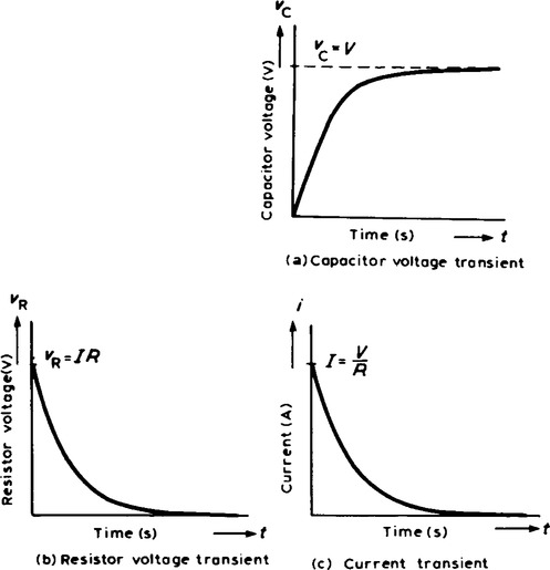
(f) Curves showing the changes in vc, vR and i with time are shown in Figure 19.2. The curve showing the variation of vc with time is called an exponential growth curve and the graph is called the ‘capacitor voltage/time’ characteristic. The curves showing the variation of vR and i with time are called exponential decay curves, and the graphs are called ‘resistor voltage/time’ and ‘current/time’ characteristics respectively. (The name ‘exponential’ shows that the shape can be expressed mathematically by an exponential mathematical equation, see para. 5 below.)
The time constant
(a) If a constant d.c. voltage is applied to a series connected C-R circuit, a transient curve of capacitor voltage vc is as shown in Figure 19.2(a).
(b) with reference to Figure 19.3, let the constant voltage supply be replaced by a variable voltage supply at time t1, seconds. Let the voltage be varied so that the current flowing in the circuit is constant.
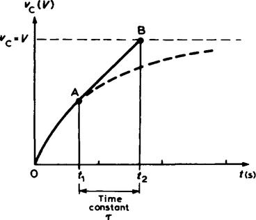
(c) Since the current flowing is a constant, the curve will follow a tangent, AB, drawn to the curve at point A.
(d) Let the capacitor voltage vc reach its final value of V at time t2 seconds.
(e) The time corresponding to (t2 − t1) seconds is called the time constant of the circuit, denoted by the Greek letter ‘tau’, τ. The value of the time constant is CR seconds, i.e. for a series connected C-R circuit, time constant, τ = CR seconds.
Since the variable voltage mentioned in para. 3(b) above can be applied at any instant during the transient change, it may be applied at t = 0, i.e. at the instant of connecting the circuit to the supply. If this is done, then the time constant of the circuit may be defined as:
‘the time taken for a transient to reach its final state if the initial rate of change is maintained’.
4. There are two main methods of drawing transient curves graphically:
(b) The initial slope and three point method which is based on the following properties of a transient exponential curve:
(i) For a growth curve, the value of a transient at a time equal to one time constant is 0.632 of its steady state value (usually taken as 63% of the steady state value); at a time equal to two and a half time constants is 0.918 of its steady state value (usually taken as 92% of its steady state value) and at a time equal to five time constants is equal to its steady state value.
(ii) For a decay curve, the value of a transient at a time equal to one time constant is 0.368 of its initial value (usually taken as 37% of its initial value), at a time equal to two and a half time constants is 0.082 of its initial value (usually taken as 8% of its initial value) and at a time equal to five time constants is equal to zero.
5. The transient curves shown in Figure 19.2 have mathematical equations, obtained by solving the differential equations representing the circuit. The equations of the curves are:
growth of capacitor voltage, υC=V(1-e−t/CR)=V(1−e−t/τ),
For example, let a 15 µF uncharged capacitor be connected in series with a 47 kω resistor across a 120 V, d.c. supply. To draw the capacitor voltage/time characteristic of the circuit using the tangential graphical method, the time constant of the circuit and the steady state value need first to be determined.

With reference to Figure 19.4, the scale of the horizontal axis is drawn so that it spans at least five time constants, i.e. 5 × 0.705 or about ![]() seconds. The scale of the vertical axis spans the change in the capacitor voltage, that is, from 0 to 120 V. A broken line All is drawn corresponding to the final value of vc.
seconds. The scale of the vertical axis spans the change in the capacitor voltage, that is, from 0 to 120 V. A broken line All is drawn corresponding to the final value of vc.
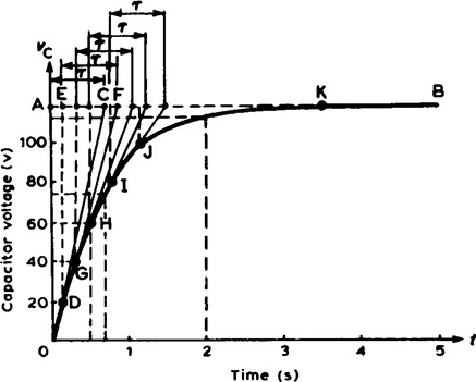
Point C is measured along AB so that AC is equal to 1τ, i.e. AC = 0.705 s. Straight line OC is drawn. Assuming that about five intermediate points are needed to draw the curve accurately, a point D is selected on OC corresponding to a vc value of about 20 V. DE is drawn vertically. EF is made to correspond to 1τ, i.e. EF = 0.705 s. A straight line is drawn joining DF. This procedure of
(a) drawing a vertical line through point selected,
(b) at the steady-state value, drawing a horizontal line corresponding to 1τ, and
is repeated for vc values of 40, 60, 80 and 100 V, giving points G, H, I and J.
The capacitor voltage effectively reaches its steady-state value of 120 V after a time equal to five time constants, shown as point K. Drawing a smooth curve through points 0, D, G, H, I, J and K gives the exponential growth curve of capacitor voltage.
From the graph, the value of capacitor voltage at a time equal to the time constant is about 75 V. It is a characteristic of all exponential growth curves, that after a time equal to one time constant, the value of the transient is 0.632 of its steady-state value. In this problem, 0.632 × 120 = 75.84 V. Also from the graph, when I is two seconds, vc is about 115 V. (This value may be checked using the equation vc = V (1 − e−t/τ, where V = 120 V, τ = 0.705 s and τ = 2 s. This calculation gives vc = 112.97 V.)
The time for vc to rise to one half of its final value, i.e. 60 V, can be determined from the graph and is about 0.5 s. This value may be checked using vc = V (1 − e-t/τ where V = 120 V, vc = 60 V and τ = 0.705 s, giving t = 0.489 s.
As another example, let a 4 µF capacitor be charged to 24 V and then discharged through a 220 kΩ resistor. To draw the capacitor voltage/time and the current/time characteristics using the ‘initial slope and three point’ method, the time constant of the circuit and the steady state value are firstly needed.
Time constant, τ = CR = 4 × 10-6 × 220 × 103 = 0.88 s.
Initially, capacitor voltage υc = υR = 24 V.

The exponential decay of capacitor voltage is from 24 V to 0 V in a time equal to five time constants, i.e. 5 × 0.88 = 4.4 s. With reference to Figure 19.5, to construct the decay curve:

(i) the horizontal scale is made so that it spans at least five time constants, i.e. 4.4 s,
(ii) the vertical scale is made to span the change in capacitor voltage, i.e. 0 to 24 V
(iii) point A corresponds to the initial capacitor voltage, i.e. 24 V,
(iv) OB is made equal to one time constant and line AB is drawn. This gives the initial slope of the transient,
(v) the value of the transient after a time equal to one time constant is 0.368 of the initial value, i.e.
A vertical line is drawn through B and distance BC is made equal to 8.83 V,
(vi) the value of the transient after a time equal to two and a half
shown as point D in Figure 19.5,
(vii) the transient effectively dies away to zero after a time equal to five time constants, i.e. 4.4 s, giving point E.
The smooth curve drawn through points A, C, D and E represents he decay transient. At 1½ s after decay has started, vC ≈ 4.4 V. This may be checked using vc = Ve-t/τ, where V = 24, t = 1½ and τ = 0.88, giving vc = 4.36 V.
The voltage drop across the resistor is equal to the capacitor voltage when a capacitor is discharging through a resistor, thus the resistor voltage/time characteristic is identical to that shown in Figure 19.5. Since vR = vc, then at 1½ seconds after decay has started,
vR ≈ 44.4 V (see above).
The current/time characteristic is constructed in the same way as the capacitor·voltage/time characteristic, and is as shown in Figure 19.6. The values are:
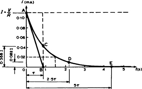
point A: initial value of current = 0.109 mA
point C: at 1τ, i = 0.368 × 0.109 = 0.040 mA
point D: at 2.5τ, i = 0.082 × 0.109=0.009 mA
Hence current transient is as shown. At a time of 1½ seconds, the value of current, from the characteristic is 0.02 mA. This may be checked using i = Ie(-t/τ) where I = 0.109, τ = 1½ and τ = 0.88, giving i = 0.0198 mA or 19.8 µA.
Discharging
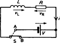
6. When a capacitor is charged (i.e. with the switch in position A in Figure 19.7), and the switch is then moved to position B, the electrons stored in the capacitor keep the current flowing for a short time. Initially, at the instant of moving from A to B, the current flow is such that the capacitor voltage vc is balanced by an equal and opposite voltage vR = iR.

Since initially vc = vR = V, then i = I = V/R.
During the transient decay, by applying Kirchhoff’s voltage law to Figure 19.7 vc = vR. Finally the transients decay exponentially to zero, i.e. vC = vR = 0. The transient curves representing the voltages and current are as shown in Figure 19.8.

Transients in series connected L-R circuits
8. When a d.c. voltage is connected to a circuit having inductance L connected in series with resistance R, there is a short period of time immediately after the voltage is connected, during which the current flowing in the circuit and the voltages across L and R are changing. These changing values are called transients.
Current growth
(a) The circuit diagram for a series connected L-R circuit is shown in Figure 19.9. When switch S is closed, then by Kirchhoff’s voltage law:
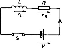
(b) The battery voltage V is constant. The voltage of the inductance is the induced voltage, i.e.
shown as L(di/dt). The voltage drop across R, VR is given by iR. Hence, at all times: V = L(di/dt) + iR.
(c) At the instant of closing the switch, the rate of change of current is such that it induces an e.m.f. in the inductance which is equal and opposite to V, hence V = vL + 0, i.e. vL = V. From equation (3), because vL = V, then vR = 0 and i = 0.
(d) A short time later at time t1 seconds after closing S, current i1 is flowing, since there is a rate of change of current initially, resulting in a voltage drop cf i1R across the resistor. Since V (constant) = vL + vR the induced e.m.f. is reduced and equation (4) becomes:
(e) A short time later still, say at time t2 seconds after closing the switch, the current flowing is i2, and the voltage drop across the resistor increases to i2R. Since vR increases, vL. decreases.
(f) Ultimately, some time after closing S, the current flow is entirely limited by R, the rate of change of current is zero and hence vL is zero. Thus V = iR. Under these conditions, steady state current flows, usually signified by I. Thus, I = V/R, vR = IR and vL = 0, at steady state conditions.
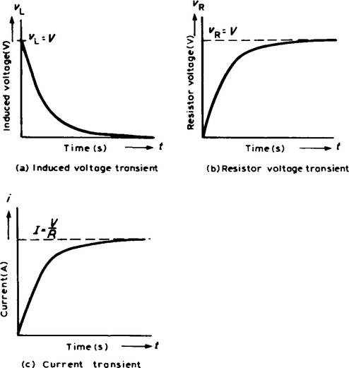
(g) Curves showing the changes in vL, vR and i with time are shown in Figure 19.10 and indicate that vL, is a maximum value initially (i.e. equal to V), decaying exponentially to zero, whereas vR and i grow from zero to their steady state values of V and I = V/R respectively.
The time constant
10. With reference to para. 3, the time constant of a series connected L-R circuit is defined in the same way as the time constant for a series connected C-R circuit. Its value is given by:
11. Transient curves representing the induced voltage/time, resistor voltage/time and current/time characteristics may be drawn graphically, as outlined in para. 4.
12. Each of the transient curves shown in Figure 19.10 have mathematical equations, and these are:
decay of induced voltage, υL=Ve(−Rt/L)=Ve(−t/τ),
Current decay
13. When a series connected L-R circuit is connected to a d.c. supply as shown with S in position A of Figure 19.11, a current I = V/R flows after a short time, creating a magnetic field (π∝I) associated with the inductor. When S is moved to position B, the current value decreases, causing a decrease in the strength of the magnetic field. Flux linkages occur, generating a voltage vL, equal to L(di/dt). Thus vL = vR
The current decays exponentially to zero and since vR is proportional to the current flowing, vR decays exponentially to zero. Since vL = vR, vL also decays exponentially to zero. The curves representing these transients are similar to those shown in Figure 19.8.
The effects of time constant on a rectangular wave
15. By varying the value of either C or R in a series connected C-R circuit, the time constant (τ = CR), of a circuit can be varied. If a rectangular waveform varying from + E to − E is applied to a C-R circuit, as shown in Figure 19.12, output waveforms of the capacitor voltage have various shapes, depending on the value of R. When R is small, τ = CR is small and an output waveform such as that shown in Figure 19.13(a) is obtained.

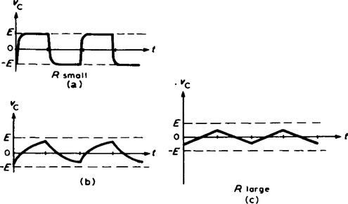
As the value of R is increased, the waveform changes to that shown in Figure 19.13(b). When R is large, the waveform is as shown in Figure 19.13(c), the circuit then being described as an integrator circuit.
16 If a rectangular waveform varying from + E to - E is applied to a series connected C-R circuit and the waveform of the voltage drop across the resistor is observed, as shown in Figure 19.14, the output waveform alters as R is varied due to the time constant, (τ = CR), altering. When R is small, the waveform is as shown in Figure 19.15(a), the voltage being generated across R by the capacitor discharging fairly quickly.
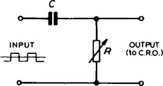
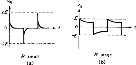
Since the change in capacitor voltage is from + E to - E, the change in discharge current is 2E/R, resulting in a change in voltage across the resistor of 2E. This circuit is called a differentiator circuit. When R is large, the waveform is as shown in Figure 19.15(b).