Electrical measuring instruments and measurements
Publisher Summary
This chapter focuses on electrical measuring instruments and measurements. To detect electrical quantities, such as current, voltage, resistance or power, it is necessary to transform an electrical quantity or condition into a visible indication. This is done with the aid of instruments (or meters) that indicate the magnitude of quantities either by the position of a pointer moving over a graduated scale, known as an analog instrument, or in the form of a decimal number, known as a digital instrument. All analog electrical indicating instruments require three essential devices, namely, a deflecting or operating device, a controlling device, and a damping device. There is no difference between the basic instrument used to measure current and voltage as both uses a milli ammeter as their basic part. This is a sensitive instrument that gives FSD for currents of only a few milli amperes. When an ammeter is required to measure currents of larger magnitude, a proportion of the current is diverted through a low value resistance connected in parallel with the meter. Such a diverting resistance is called a shunt.
1. Tests and measurements are important in designing, evaluating, maintaining and servicing electrical circuits and equipment. In order to detect electrical quantities such as current, voltage, resistance or power, it is necessary to transform an electrical quantity or condition into a visible indication. This is done with the aid of instruments (or meters) that indicate the magnitude of quantities either by the position of a pointer moving over a graduated scale (called an analogue instrument) or in the form of a decimal number (called a digital instrument).
2. All analogue electrical indicating instruments require three essential devices. These are:
(a) A deflecting or operating device A mechanical force is produced by the current or voltage which causes the pointer to deflect from its zero position.
(b) A controlling device The controlling force acts in opposition to the deflecting force and ensures that the deflection shown on the meter is always the same for a given measured quantity. It also prevents the pointer always going to the maximum deflection. There are two main types of controlling device — spring control and gravity control.
(c) A damping device The damping force ensures that the pointer comes to rest in its final position quickly and without undue oscillation. There are three main types of damping used — eddy-current damping, air-friction damping and fluid-friction damping.
3. There are basically two types of scale — linear and non-linear. A linear scale is shown in Figure 23.1(a) where each of the divisions or graduations are evenly spaced. The voltmeter shown has a range 0–100 V, i.e. a full scale deflection (FSD) of 100 V.

A non-linear scale is shown in Figure 23.1(b). The scale is cramped at the beginning and the graduations are uneven throughout the range. The ammeter shown has a FSD of 10 A.
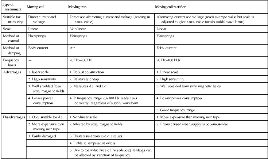
4 A comparison of measuring instruments is shown in the table on pages 198 and 199.
Principle of operation of a moving coil instrument
5. A moving coil instrument operates on the motor principle. When a conductor carrying current is placed in a magnetic field, a force F is exerted on the conductor, given by F = BIl. If the flux density B is made constant (by using permanent magnets) and the conductor is a fixed length (say, a coil) then the force will depend only on the current flowing in the conductor.
In a moving coil instrument, a coil is placed centrally in the gap between shaped pole pieces as shown by the front elevation in Figure 23.2(a). The coil is supported by steel pivots, resting in jewel bearings, on a cylindrical iron core. Current is led into and out of the coil by two phosphor bronze spiral hairsprings which are wound in opposite directions to minimise the effect of temperature change and to limit the coil swing (i.e. to control the movement) and return the movement to zero position when no current flows.

Current flowing in the coil produces forces as shown in Figure 23.2(b), the directions being obtained by Fleming’s left-hand rule. The two forces, FA and FB, produce a torque which will move the coil in a clockwise direction, i.e. move the pointer from left to right. Since force is proportional to current the scale is linear.
When the aluminium frame, on which the coil is wound, is rotated between the poles of the magnet, small currents (called eddy currents) are induced into the frame, and this provides automatically the necessary damping of the system due to the reluctance of the former to move within the magnetic field.
The moving coil instrument will only measure direct current or voltage and the terminals are marked positive and negative to ensure that the current passes through the coil in the correct direction to deflect the pointer ’up the scale’.
The range of this sensitive instrument is extended by using shunts and multipliers. (See para. 10.)
Comparison of the moving coil, moving iron and moving coil rectifier instruments
| Type of instrument | Moving coil | Moving iron | Moving coil rectifier |
| Suitable for measuring. | Direct current and voltage. | Direct and alternating current and voltage (reading in r.m.s. value). | Alternating current and voltage (reads average value but scale is adjusted to give r.m.s. value for sinusoidal waveforms). |
| Scale | Linear | Non-linear | Linear |
| Method of control | Hairsprings | Hairsprings | Hairsprings |
| Method of damping | Eddy current | Air | Eddy current |
| Frequency limits | — | 20 Hz–200 Hz | 20 Hz–100 kHz |
| Advantages | 1. linear scale. | 1. Robust construction. | 1. Linear scale. |
| 2. High sensitivity. | 2. Relatively cheap. | 2. High sensitivity. | |
| 3. Well shielded from stray magnetic fields. | 3. Measures d.c. and a.c. | 3. Well shielded from stray magnetic fields. | |
| 4. Lower power consumption. | 4. In frequency range 20–100 Hz reads r.m.s. correctly, regardless of supply waveform. | 4. Lower power consumption. | |
| 5. Good frequency range. | |||
| Disadvantages | 1. Only suitable for d.c. | 1 Non-linear scale. | 1. More expensive than moving iron type. |
| 2. More expensive than moving iron type. | 2 Affected by stray magnetic fields. | 2. Errors caused when supply is non-sinusoidal. | |
| 3. Easily damaged. | 3. Hysteresis errors in d.c. circuits. | ||
| 4. Liable to temperature errors. | |||
| 5. Due to the inductance of the solenoid, readings can be affected by variation of frequency. |
Principle of operation of the moving iron instrument
(a) An attraction type of moving iron instrument is shown diagrammatically in Figure 23.3(a). When current flows in the solenoid, a pivoted soft iron disc is attracted towards the solenoid and the movement causes a pointer to move across a scale.
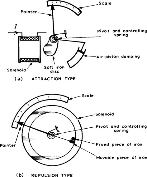
(b) In the repulsion type moving iron instrument shown diagrammatically in Figure 23.3(b), two pieces of iron are placed inside the solenoid, one being fixed, and the other attached to the spindle carrying the pointer.
When current passes through the solenoid, the two pieces of iron are magnetised in the same direction and therefore repel each other. The pointer thus moves across the scale. The force moving the pointer is, in each type, proportional to I2. Because of this the direction of current does not matter and the moving iron instrument can be used on d.c. or a.c. The scale, however, is non-linear.
7. A moving coil instrument, which measures only d.c., may be used in conjunction with a bridge rectifier circuit as shown in Figure 23.4 to provide an indication of alternating currents and voltages. The average value of the full wave rectified current is
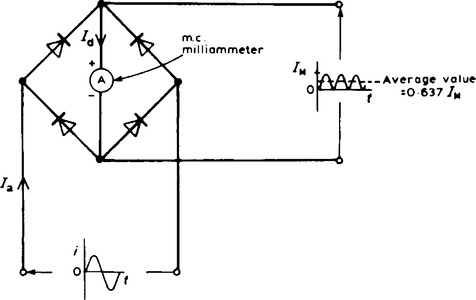
0.637 IM. However, a meter being used to measure a.c. is usually calibrated in r.m.s. values. For sinusoidal quantities the indication is 0.707 IM/0.637 IM, i.e. 1.11 times the mean value.
Rectifier instruments have scales calibrated in r.m.s. quantities and it is assumed by the manufacturer that the a.c. is sinusoidal.
Shunts and multipliers
10. There is no difference between the basic instrument used to measure current and voltage since both use a milliammeter as their basic part. This is a sensitive instrument which gives FSD for currents of only a few milliamperes. When an ammeter is required to measure currents of larger magnitude, a proportion of the current is diverted through a low value resistance connected in parallel with the meter. Such a diverting resistance is called a shunt.
From Figure 23.5(a), VPQ = VRS.

The milliammeter is converted into a voltmeter by connecting a high resistance (called a multiplier) in series with it as shown in Figure 23.5(a). From Figure 23.5(b), V = Va + VM = Ira + IRM
Thus the value of the multiplier, RM=V—Ira/I Ω.
For example, let a m.c. instrument have a FSD of 20 mA and a resistance of 25 Ω. To enable the instrument to be used as a 0—10 A ammeter, a shunt resistance RS needs to be connected in parallel with the instrument. From Figure 23.5(a),
Hence the value of RS is given by:
To enable the instrument to be used as a 0 to 100 V voltmeter, a multiplier RM needs to be connected in series with the instrument, the value of RM being given by:
11. An ohmmeter is an instrument for measuring electrical resistance. A simple ohmmeter circuit is shown in Figure 23.6(a). Unlike the ammeter or voltmeter, the ohmmeter circuit does not receive the energy necessary for its operation from the circuit under test. In the ohmmeter this energy is supplied by a self-contained source of voltage, such as a battery. Intially, terminals XX are short-circuited and R adjusted to give FSD on the milliammeter. If current I is at a maximum value and voltage E is constant, then resistance R=E/I is at a minimum value. Thus FSD on the milliammeter is made zero on the resistance scale. When terminals XX are open circuited no current flows and R (=E/O) is infinity, ∞. The milliammeter can thus be calibrated directly in ohms. A cramped (non-linear) scale results and is ’back to front’ (as shown in Figure 23.6(b)). When calibrated, an unknown resistance is placed between terminals XX and its value determined from the position of the pointer on the scale. An ohmmeter designed for measuring low values of resistance is called a continuity tester. An ohmmeter designed for measuring high values of resistance (i.e. megohms) is called an insulation resistance tester (or ’megger’).

12. Instruments are manufactured that combine a moving coil meter with a number of shunts and series multipliers, to provide a range of readings on a single scale graduated to read current and voltage. If a battery is incorporated into the instrument then resistance can also be measured.
Such instruments are called multimeters or universal instruments or multirange instruments. An Avometer is a typical example. A particular range may be selected either by the use of separate terminals or by a selector switch. Only one measurement can be performed at one time. Often such instruments can be used in a.c. as well as d.c. circuits when a rectifier is incorporated in the instrument.
13. A wattmeter is an instrument for measuring electrical power in a circuit. Figure 23.7 shows typical connections of a wattmeter used for measuring power supplied to a load. The instrument has two coils:
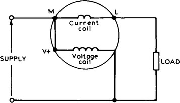
(i) a current coil, which is connected in series with the load (like an ammeter), and
(ii) a voltage coil, which is connected in parallel with the load (like a voltmeter).
14. The cathode ray oscilloscope (CRO) may be used in the observation of waveforms and for the measurement of voltage, current, frequency, phase and periodic time.
(i) With direct voltage measurements, only the Y amplifier ’volts/cm’ switch on the CRO is used. With no voltage applied to the Y plates the position of the spot trace on the screen is noted. When a direct voltage is applied to the Y plates the new position of the spot trace is an indication of the magnitude of the voltage. For example, in Figure 23.8(a), with no voltage applied to the Y plates, the spot trace is in the centre of the screen (initial position) and then the spot trace moves 2.5 cm to the final position shown, on application of a d.c. voltage. With the ’V/cm’ switch on 10 V/cm the magnitude of the direct voltage is 2.5 cm × 10 V/cm, i.e. 25 V.
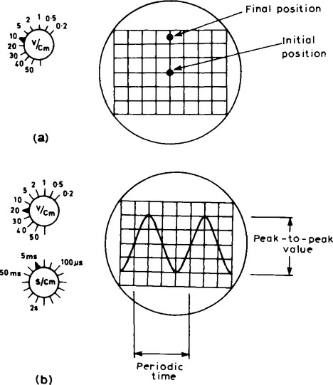
(ii) With alternating voltage measurements, let a sinusoidal waveform be displayed on a CRO screen as shown in Figure 23.8(b). If the ’variable’ switch is on, say, 5 ms/cm then the periodic time T of the sine wave is 5 ms/cm × 4 cm, i.e. 20 ms or 0.02 s.
If the ’volts/cm’ switch is on, say, 20 V/cm then the amplitude or peak value of the sine wave shown is 20 V/cm × 2 cm, i.e. 40 V.
Double beam oscilloscopes are useful whenever two signals are to be compared simultaneously. The CRO demands reasonable skill in adjustment and use. However its greatest advantage is in observing the shape of a waveform — a feature not possessed by other measuring instruments.
15. An electronic voltmeter can be used to measure with accuracy e.m.f or p.d. from millivolts to kilovolts by incorporating in its design amplifiers and attentuators.
16. A null method of measurement is a simple, accurate and widely used method which depends on an instrument reading being adjusted to read zero current only. The method assumes:
Hence it is unnecessary for a meter sensing current flow to be calibrated when used in this way. A sensitive milliammeter or microammeter with centre zero position setting is called a galvanometer. Two examples where the method is used are in the Wheatstone bridge and in the d.c. potentiometer.
17. A Wheatstone bridge, shown in Figure 23.9, is used in d.c. circuits to compare an unknown resistance Rx with others of known values. R3 is varied until zero deflection is obtained on the galvanometer, G. At balance (i.e. zero deflection on the galvanometer) the products of diagonally opposite resistances are equal to one another,

18. The d.c. potentiometer is a null-balance instrument used for determining values of e.m.f’s and p.d.’s by comparison with a known e.m.f. or p.d. In Figure 23.10(a), using a standard cell of known e.m.f. E1, the slider S is moved along the slide wire until balance is obtained (i.e. the galvanometer deflection is zero), shown as length l1. The standard cell is now replaced by a cell of unknown e.m.f., E2 (see Figure 21.10(b)) and again balance is obtained (shown as l2). Since E1 ∝ l1 and E2 ∝ l2,

A.C. bridges
19. A Wheatstone bridge type circuit, shown in Figure 23.11, may be used in a.c. circuits to determine unknown values of inductance and capacitance, as well as resistance. When the potential differences across Z3 and Zx (or across Z1 and Z2) are equal in magnitude and phase, then the current flowing through the galvanometer, G, is zero. At balance, Z1Zx = Z2Z3, from which
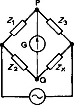
20. There are many forms of a.c. bridge, and these include: the Maxwell, Hay, Owen and Heaviside bridges for measuring inductance, and the De Sauty, Schering and Wien bridges for measuring capacitance. A commercial or universal bridge is one which can be used to measure resistance, inductance or capacitance.
21. Maxwell’s bridge for measuring the inductance L and resistance r of an inductor is shown in Figure 23.12.

Equating the real parts gives: R1R2R3 = R3XCXL
Equating the imaginary parts gives:
From equation (1), R2=L/R1C and from
equation (2), R3 = R1/rR2. Hence ![]()
If the frequency is constant then
Thus the bridge can be adjusted to give a direct indication of Q-factor.
(see Chapter 13, para. 15).
The simplified circuit of a Q-meter, used for measuring Q-factor, is shown in Figure 23.13. Current from a variable frequency oscillator flowing through a very low resistance r develops a variable frequency voltage, Vr, which is applied to a series L-R-C circuit. The frequency is then varied until resonance causes voltage Vc to reach a maximum value. At resonance Vr and Vc are noted.
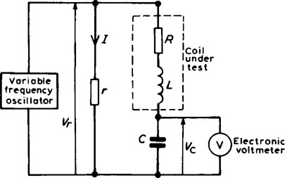
In a practical Q-meter, Vr is maintained constant and the electronic voltmeter can be calibrated to indicate the Q-factor directly. If a variable capacitor C is used and the oscillator is set at a given frequency, then C can be adjusted to give resonance. In this way inductance L may be calculated using
Since Q=2πfL/R, then R may be calculated.
Q-meters operate at various frequencies and instruments exist with frequency ranges from 1 kHz to 50 MHz. Errors in measurement can exist with Q-meters since the coil has an effective parallel self capacitance due to capacitance between turns. The accuracy of a Q-meter is approximately ±5%.
Waveform harmonics
(i) Let an instantaneous voltage v be represented by v = VM sin 2πft volts. This is a waveform which varies sinusoidally with time t, has a frequency f, and a maximum value, VM. Alternating voltages are usually assumed to have wave-shapes which are sinusoidal where only one frequency is present. If the wave-form is not sinusoidal it is called a complex wave, and, whatever its shape, it may be split up mathematically into components called the fundamental and a number of harmonics. This process is called harmonic analysis. The fundamental (or first harmonic) is sinusoidal and has the supply frequency, f, the other harmonics are also sine waves having frequencies which are integer multiples of f. Thus, if the supply frequency is 50 Hz, then the third harmonic frequency is 150 Hz, the fifth 250 Hz, and so on.
(ii) A complex waveform comprising the sum of the fundamental and a third harmonic of about half the amplitude of the fundamental is shown in Figure 23.14(a), both waveforms being initially in phase with each other. If further odd harmonic waveforms of the appropriate amplitudes are added, a good approximation to a square wave results.
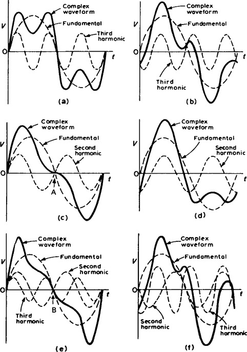
In Figure 23.14(b) the third harmonic is shown having an initial phase displacement from the fundamental. The positive and negative half cycles of each of the complex waveforms shown in Figure 23.14(a) and (b) are identical in shape, and this is a feature of waveforms containing the fundamental and only odd harmonics.
(iii) A complex waveform comprising the sum of the fundamental and a second harmonic of about half the amplitude of the fundamental is shown in Figure 23.14(c), each waveform being initially in phase with each other. If further even harmonics of appropriate amplitudes are added a good approximation to a triangular wave results. In Figure 23.14(c) the negative cycle appears as a mirror image of the positive cycle about point A. In Figure 23.14(d) the second harmonic is shown with an initial phase displacement from the fundamental and the positive and negative half cycles are dissimilar.
(iv) A complex waveform comprising the sum of the fundamental, a second harmonic and a third harmonic is shown in Figure 23.14(e), each waveform being initially ’in-phase’. The negative half cycle appears as a mirror image of the positive cycle about point B. In Figure 23.14(f), a complex waveform comprising the sum of the fundamental, a second harmonic and a third harmonic, are shown with initial phase displacement. The positive and negative half cycles are seen to be dissimilar.
The features mentioned relative to Figures 23.14(a) to (f) make it possible to recognise the harmonics present in a complex waveform displayed on a CRO.
24. Some measuring instruments depend for their operation on power taken from the circuit in which measurements are being made. Depending on the ’loading’ effect of the instrument (i.e. the current taken to enable it to operate), the prevailing circuit conditions may change. The resistance of voltmeters may be calculated since each have a stated sensitivity (or ’figure of merit’), often stated in ’kω per volt’ of FSD. A voltmeter should have as high a resistance as possible (– ideally infinite). In a.c. circuits the impedance of the instrument varies with frequency and thus the loading effect of the instrument can change. Electronic measuring instruments have advantages over instruments such as the moving iron or moving coil meters, in that they have a much higher input resistance (some as high as 1000 MΩ) and can handle a much wider range of frequency (from d.c. up to MHz).
25. Instruments for a.c. measurements are generally calibrated with a sinusoidal alternating waveform to indicate r.m.s. values when a sinusoidal signal is applied to the instrument. Some instruments, such as the moving iron and electrodynamic instruments, give a true r.m.s. indication. With other instruments the indication is either scaled up from the mean value (such as with the rectifier moving coil instrument) or scaled down from the peak value. Sometimes quantities to be measured have complex waveforms (see para. 23), and whenever a quantity is non-sinusoidal, errors in instrument readings can occur if the instrument has been calibrated for sine waves only. Such waveform errors can be largely eliminated by using electronic instruments.
26. Errors are always introduced when using instruments to measure electrical quantities. Besides possible errors introduced by the operator or by the instrument disturbing the circuit, errors are caused by the limitations of the instrument used.
The calibration accuracy of an instrument depends on the precision with which it is constructed. Every instrument has a margin of error which is expressed as a percentage of the instruments full scale deflection. For example, an instrument may have an accuracy of ±2% of FSD. Thus, if a voltmeter has a FSD of 100 V and it indicates say 60 V, then the actual voltage measured may be anywhere between 60 V± (2% of 100 V), i.e. 60±2 V, i.e. between 58 V and 62 V. As a percentage of the voltmeter reading this error is ±2/60 × 100%, i.e. ±3.33%. Hence the accuracy can be expressed as 60 V ±3.33%. It follows that an instrument having a 2% FSD accuracy can give relatively large errors when operating at conditions well below FSD.
When more than one instrument is used in a circuit then a cumulative error results. For example, if the current flowing through and the p.d. across a resistor is measured, then the percentage error in the ammeter is added to the percentage error in the voltmeter when determining the maximum possible error in the measured value of resistance.
Decibel units
27. In electronic systems, the ratio of two similar quantities measured at different points in the system, are often expressed in logarithmic units. By definition, if the ratio of two powers P1 and P2 is to be expressed in decibel (dB) units then the number of decibels, X, is given by:
Thus, when the power ratio, P2/P1=1,
then the decibel power ratio= 10 lg 1=0
when the power ratio, P2/P1=100,
then the decibel power ratio= 10 lg 100= + 20
and when the power ratio, P2/P1 =1/10,
then the decibel power ratio= 10 lg 1/10= — 10,
(i.e. a power loss or attentuation).
28 Logarithmic units may also be used for voltage and current ratios. Power P, is given by P = I2R or P=V2/R.
Substituting in equation (1) gives:
(from the laws of logarithms).
Thus if the current input to a system is 5 mA and the current output is 20 mA, the decibel current ratio
29. From equation (1), X decibels is a logarithmic ratio of two similar quantities and is not an absolute unit of measurement. It is therefore necessary to state a reference level to measure a number of decibels above or below that reference. The most widely used reference level for power is 1 mW, and when power levels are expressed in decibels, above or below the 1 mW reference level, the unit given to the new power level is dBm.
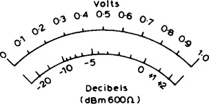
A voltmeter can be re-scaled to indicate the power level directly in decibels. The scale is generally calibrated by taking a reference level of 0 dB when a power of 1 mW is dissipated in a 600Ω resistor (this being the natural impedance of a simple transmission line). The reference voltage V is then obtained from
In general, the number of dBm, X=20 lg ![]() .
.
Thus V=0.20 V corresponds to 20 lg ![]() = —11.77 dBm and
= —11.77 dBm and
V=0.90 V corresponds to 20 lg ![]() = + 1.3 dBm, and so on.
= + 1.3 dBm, and so on.
A typical decibelmeter, or dB meter scale is shown in Figure 23.15. Errors are introduced with dB meters when the circuit impedance is not 600 Ω.