Alternating currents and voltages
Publisher Summary
This chapter focuses on alternating currents and voltages. Electricity is produced by generators at power stations and then distributed by a vast network of transmission lines to industry and for domestic use. It is easier and cheaper to generate alternating current (a.c.) than direct current (d.c.), and a.c. is more conveniently distributed than d.c. as its voltage can be readily altered using transformers. The effective value of an alternating current is that current that will produce the same heating effect as an equivalent direct current. The effective value is called the root mean square (r.m.s.) value and whenever an alternating quantity is given, it is assumed to be the r.m.s. value. The process of obtaining unidirectional currents and voltages from alternating currents and voltages is called rectification. Automatic switching in circuits is carried out by devices called diodes.
1. Electricity is produced by generators at power stations and then distributed by a vast network of transmission lines (called the National Grid system) to industry and for domestic use. It is easier and cheaper to generate alternating current (a.c.) than direct current (d.c.) and a.c. is more conveniently distributed than d.c. since its voltage can be readily altered using transformers. Whenever d.c. is needed in preference to a.c. devices called rectifiers are used for conversion (see paragraphs 19 to 23).
2. Let a single turn coil be free to rotate at constant angular velocity ω symmetrically between the poles of a magnet system as shown in Figure 12.1. An emf is generated in the coil (from Faraday’s law) which varies in magnitude and reverses its direction at regular intervals. The reason for this is shown in Figure 12.2. In positions (a), (e) and (i) the conductors of the loop are effectively moving along the magnetic field, no flux is cut and hence no emf is induced. In position (c) maximum flux is cut and hence maximum emf is induced. In position (g), maximum flux is cut and hence maximum emf is again induced. However, using Fleming’s right-hand rule, the induced emf is in the opposite direction to that in position (c) and is thus shown as –E. In positions (b), (d), (f) and (h) some flux is cut and hence some emf is induced. If all such positions of the coil are considered, in one revolution of the coil, one cycle of alternating emf is produced as shown. This is the principle of operation of the a.c. generator (i.e. the alternator).


3. If values of quantities which vary with time t are plotted to a base of time, the resulting graph is called a waveform. Some typical waveforms are shown in Figure 12.3. Waveforms (a) and (b) are unidirectional waveforms, for, although they vary considerably with time, they flow in one direction only (i.e. they do not cross the time axis and become negative). Waveforms (c) to (g) are called alternating waveforms since their quantities are continually changing in direction (i.e. alternately positive and negative).
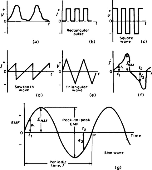
4. A waveform of the type shown in Figure 12.3(g) is called a sine wave It is the shape of the waveform of emf produced by an alternator and thus the mains electricity supply is of ‘sinusoidal’ form.
5. One complete series of values is called a cycle (i.e. from O to P in Figure 12.3(g)).
6. The time taken for an alternating quantity to complete one cycle is called the period or the periodic time, T, of the waveform.
7. The number of cycles completed in one second is called the frequency, f, of the supply and is measured in hertz, Hz. The standard frequency of the electricity supply in Great Britain is 50 Hz.
8. Instantaneous values are the values of the alternating quantities at any instant of time. They are represented by small letters, i, v, e etc. (see Figure 12.3(f) and (g)).
9. The largest value reached in a half cycle is called the peak value or the maximum value or the crest value or the amplitude of the waveform. Such values are represented by VMAX, IxMAX etc. (see Figure 12.3(f) and (g)). A peak-to-peak value of emf is shown in Figure 12.3(g) and is the difference between the maximum and minimum values in a cycle.
10. The average or mean value of a symmetrical alternating quantity, (such as a sinewave), is the average value measured over a half cycle, (since over a complete cycle the average value is zero).
The area under the curve is found by approximate methods such as the trapezoidal rule, the mid-ordinate rule or Simpson’s rule. Average values are represented by VAV, IAV, etc.
For a sine wave, average value = 0.637 × maximum value![]() .
.
11. The effective value of an alternating current is that current which will produce the same heating effect as an equivalent direct current. The effective value is called the root mean square (r.m.s.) value and whenever an alternating quantity is given, it is assumed to be the r.m.s. value. For example, the domestic mains supply in Great Britain is 240 V and is assumed to mean ‘240 V r.m.s.’. The symbols used for r.m.s. values are I, V, E, etc. For a non-sinusoidal waveform as shown in Figure 12.4, the r.m.s. value is given by:

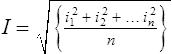
where n is the number of intervals used.
For a sine wave, r.m.s. value = 0.707 × maximum value.
The values of form and peak factors give an indication of the shape of waveforms.
13. In Figure 12.5, OA represents a vector that is free to rotate anticlockwise about 0 at an angular velocity of ω rad/s. A rotating vector is known as a phasor. After time t seconds the vector OA has turned through an angle ωt. If the line BC is constructed perpendicular to OA as shown, then
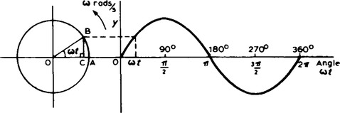
If all such vertical components are projected on to a graph of y against angle ωt (in radians), a sine curve results of maximum value OA. Any quantity which varies sinusoidally can thus be represented as a phasor.
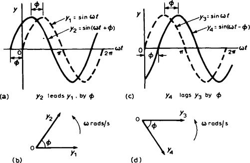
14. A sine curve may not always start at 0°. To show this a periodic function is represented by y = sin(ωt±ϕ), where ϕ is a phase (or angle) difference compared with y = sin ωt. In Figure 12.6(a), y2 = sin (ωt + ϕ) starts ϕ radians earlier than y1 = sin ωt and is thus said to lead y1 by ϕ radians. Phasors y1 and y2 are shown in Figure 12.6(b) at the time when t = 0. In Figure 12.6(c), y4 = sin(ωt – ϕ) starts ϕ radians later than y3 = sin ωt and is thus said to lag y3 by ϕ radians. Phasors y3 and y4 are shown in Figure 12.6(d) at the time when t = 0.
15. Given the general sinusoidal voltage, V = VMAX sin (ωt±ϕ), then
(i) Amplitude or maximum value = VMAX;
(ii) Peak to peak value = 2 VMAX;
(iii) Angular velocity = ω rad/s.
(v) Frequency, ![]() Hz (hence ω=2πf).
Hz (hence ω=2πf).
(vi) ϕ = angle of lag or lead (compared with v = VMAX sin ωt).
16. The resultant of the addition (or subtraction) of two sinusoidal quantities may be determined either:
For example, currents i1 = 20 sin ωt and i2 = 10 sin![]() are shown plotted in Figure 12.7.
are shown plotted in Figure 12.7.
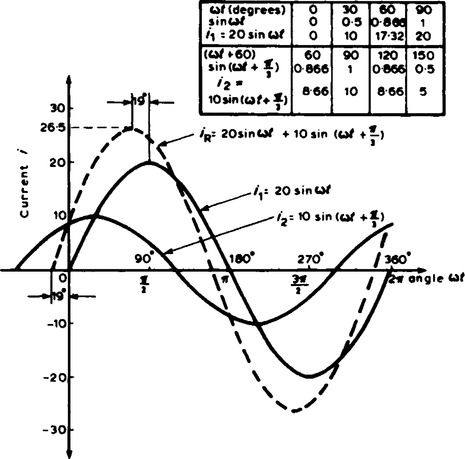
To determine the resultant of i1 + i2, ordinates of i1 and i2 are added at, say, 15° intervals. For example:
at 30°, i1 + i2 = 10 + 10=20 A
at 60°, i1 + i2 = 8.7 + 17.3=26 A
at 150°, + i1 + i2 = 10 + (– 5) = 5 A, and so on.
The resultant waveform for i1 + i2 is shown by the broken line in Figure 12.7. It has the same period, and hence frequency, as i1 and i2. The amplitude or peak value is 26.5 A. The resultant waveform leads i1 = 20 sin ωt by 19°, i.e., ![]() rad = 0.332 rad. Hence the sinusoidal expression for the resultant i1 + i2 is given by: iR = i1 + i2 = 26.5 sin(ωt + 0.332) A.
rad = 0.332 rad. Hence the sinusoidal expression for the resultant i1 + i2 is given by: iR = i1 + i2 = 26.5 sin(ωt + 0.332) A.
The relative positions of i1 and i2 at time = 0 are shown as phasors in Figure 12.8(a). The phasor diagram in Figure 12.8(b) shows the resultant iR, and iR is measured as 26 A and angle ϕ as 19° (i.e. 0.33 rad) leading i1. Hence, by drawing, iR = 26 sin(ωt + 0.33) A. From Figure 12.8(b), by the cosine rule:
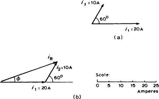
from which, iR = 26.46 A. By the sine rule:
from which, ϕ = 19° 10’ (i.e., 0.333 rad).
Hence, by calculation, iR = 26.46 sin(ωt + 0.333) A.
17. When a sinusoidal voltage is applied to a purely resistive circuit of resistance R, the voltage and current waveforms are in phase and I = ![]() (exactly as in d.c. circuit). V and I are r.m.s. values.
(exactly as in d.c. circuit). V and I are r.m.s. values.
18. For an a.c. resistive circuit, power ![]() watts (exactly as in a d.c. circuit). V and I are r.m.s. values.
watts (exactly as in a d.c. circuit). V and I are r.m.s. values.
19. The process of obtaining unidirectional currents and voltages from alternating currents and voltages is called rectification. Automatic switching in circuits is carried out by devices called diodes (see page 130).
20. Using a single diode, as shown in Figure 12.9, half-wave rectification is obtained. When P is sufficiently positive with respect to Q diode D is switched on and current i flows.
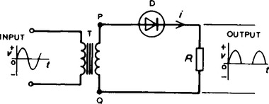
When P is negative with respect to Q diode D is switched off. Transformer T isolates the equipment from direct connection with the mains supply and enables the mains voltage to be changed.
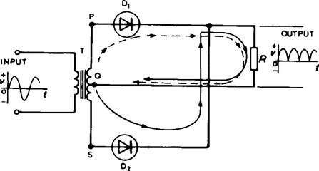
21. Two diodes may be used as shown in Figure 12.10 to obtain full wave rectification. A centre-tapped transformer T is used. When P is sufficiently positive with respective to Q diode D1 conducts and current flows (shown by the broken line in Figure 12.10). When S is positive with respect to Q, diode D2 conducts and current flows (shown by continuous line in Figure 12.10). The current flowing in R is in the same direction for both half cycles of the input. The output waveform is thus as shown in Figure 12.10.
22. Four diodes may be used in a bridge rectifier circuit, as shown in Figure 12.11 to obtain full wave rectification. As for the rectifier shown in Figure 12.10, the current flowing in R is in the same direction for both half cycles of the input giving the output waveform shown.

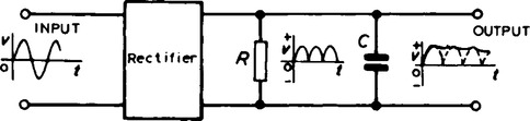
23. To smooth the output of the rectifiers described above, capacitors having a large capacitance may be connected across the load resistors R. The effect of this is shown on the output in Figure 12.12.