
a.c. circuit analysis
Publisher Summary
This chapter focuses on the analysis of alternating current (a.c.) circuit. Circuit theory and the analysis of a.c. circuits is invariably achieved by using complex numbers—otherwise known as symbolic or jnotation. The effect of multiplying a phasor by j is to rotate it in a positive direction, that is, anticlockwise, on an Argand diagram through 90° without altering its length. Similarly, multiplying a phasor by—j rotates the phasor through—90°. These facts are used in the a.c. theory as certain quantities in the phasor diagrams lie at 90° to each other. There are a number of circuit theorems that have been developed for solving problems in a.c. electrical networks. These include the superposition theorem, Thévénins theorem, Norton’s theorem, and the maximum power transfer theorem. As a preliminary to using circuit theorems, star-delta and delta-star transformations can be used.
1. The laws which determine the currents and voltage drops in a.c. circuits are:
(b) the laws for impedances in series and parallel, i.e., total impedance ZT = Z1 + Z2 + Z3 + · · · for impedances connected in series, ![]() for impedances connected in parallel, and
for impedances connected in parallel, and
(c) Kirchhoffs laws (as for d.c. circuits —see page 28).
2. A number such as 3+ j2 is called a complex number, the 3 being the real part and j2 the imaginary part. By definition ![]() (see Newnes Mathematics Pocket Book, page 81).
(see Newnes Mathematics Pocket Book, page 81).
Circuit theory and analysis of a.c. circuits is invariably achieved using complex numbers (otherwise known as symbolic or j notation).
The effect of multiplying a phasor by j is to rotate it in a positive direction (i.e. anticlockwise) on an Argand diagram through 90° without altering its length. Similarly, multiplying a phasor by −j rotates the phasor through 90°. These facts are used in a.c. theory since certain quantities in the phasor diagrams lie at 90° to each other. For example, in the R-L series circuit shown in Figure 15.1(a), VL leads I by 90° (i.e. I lags VL by 90°) and may be written as jVL, the vertical axis being regarded as the imaginary axis of an Argand diagram. Thus VR + jVL = V and since VR = IR, VL = IXL and V = IZ, then R + jXL = Z.

Similarly, for the R-C circuit shown in Figure 15.1(b), VC lags I by 90° (i.e. I leads VC by 90°) and VR – jVC = V, from which R – jXC = Z. Thus an impedance of (3 + j2) ohms represents a resistance of 3 Ω in series with an inductance of inductive reactance XL of 2 Ω and an impedance of (5– j7) Ω represents a resistance of 5 Ω in series with a capacitance of capacitive reactance 7 Ω.
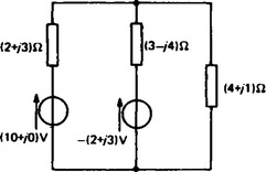
For example, to determine the current flowing in the (4 + j1) Ω impedance in Figure 15.2, currents are initially assigned to the three branches, as shown by i1, i2 and (i1 + i2).
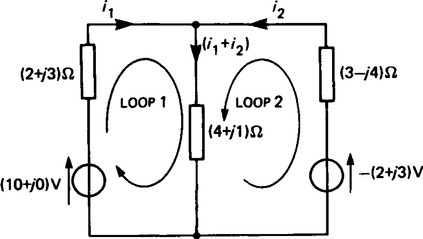
 (1)
(1) (2)
(2)To eliminate i2, equation (1) is multiplied by (7−j3) and equation (2) by (4+ j1).
Equation (3)–equation (4) gives:
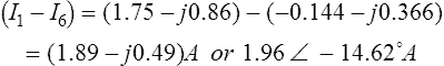
From equation (1), 10= (1.89−j0.51)(6+ j4)+ i2(4+ j1)

Thus (i1 + u2) = (1.89−j0.51) + (−1.06−j0.86) = (0.83− j1.37)A or 1.60 ∠-59°A.
3. There are a number of circuit theorems which have been developed for solving problems in a.c. electrical networks. These include:
As a preliminary to using circuit theorems, star-delta and delta-star transformations may be used.
‘In any network made up of linear impedances and containing more than one source of emf, the resultant current flowing in any branch is the algebraic sum of the currents that would flow in that branch if each source was considered separately, all other sources being replaced at that time by their respective internal impedances.’
For example, to determine the current flowing in each branch of the network shown in Figure 15.2 using the superposition theorem, the procedure is:
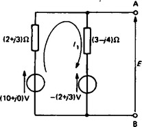
(i) Redraw the original circuit with the −(2+j3) volt source removed as shown in Figure 15.3.
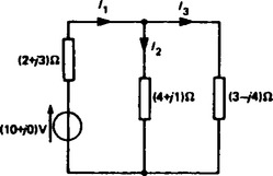
(ii) Label the currents in each branch and their directions as shown in Figure 15.3, and determine their values.
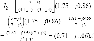
(4+ j1) Ω in parallel with (3 −j4) Ω gives an equivalent impedance of
Hence from the equivalent circuit of Figure 15.4:

From Figure 15.3,
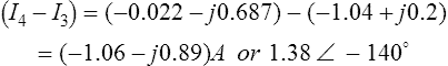
and I3 = I1− I2 = (1.75−j0.86)−(0.71 −j1.06) = (1.04 + j0.20)A.
(iii) Redraw the original circuit with the (10 + j0) volt source removed, as shown in Figure 15.5.

(iv) Label the currents in each branch and their directions as shown in Figure 15.5 and determine their values.
(2+ j3) Ω in parallel with (4+ j1) Ω gives an equivalent impedance of
From the equivalent circuit of Figure 15.6
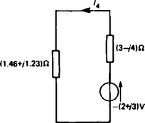
From Figure 15.5,

From Figure 15.5,

(v) Superimposing Figure 15.3 on to Figure 15.5 gives:

as shown in Figure 15.7.

(a) Thévémin’s theorem states:
‘The current in any branch of a network is that which would result if an emf, equal to the p.d. across a break made in the branch, were introduced into the branch, all other emfs being removed and represented by the internal impedances of the sources.’
(b) To determine the current in any branch of an active network the procedure adopted is:
(i) remove the impedance Z from that branch;
(ii) determine the open-circuit voltage E across the break;
(iii) remove each source of emf and replace them by their internal impedances and then determine the impedance z ‘looking-in’ at the break,
(iv) determine the value of the current from the equivalent circuit shown in Figure 15.8.

For example, to determine the current flowing in the (4+ j1) Ω impedance shown in Figure 15.9 using Thévenin’s theorem (note Figure 15.9 is the same as Figure 15.2:
(i) The impedance (4 + j1) Ω is removed as shown in Figure 15.10.

(iii) Removing the sources of emf gives the circuit of Figure 15.11, from which,


(iv) The equivalent Thévénin circuit is shown in Figure 15.12.

‘The current that flows in any branch of a network is the same as that which would flow in the branch if it were connected across a source of electricity, the short-circuit current of which is equal to the current that would flow in a short-circuit across the branch, and the internal impedance of which is equal to the impedance which appears across the open-circuited branch terminals.’
(b) To determine the current in any branch AB of an active network the procedure adopted is:
(i) short-circuit that branch;
(ii) determine the short-circuit current, ISC;
(iii) remove each source of emf and replace them by their internal impedances (or, if a current source exists replace with an open-circuit), then determine the impedance, z, looking-in’ at a break made between A and B,
(iv) determine the value of the current from the equivalent circuit shown in Figure 15.13,
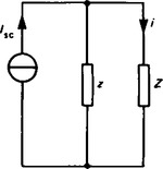
For example, to determine the current flowing in the (4+ j1) Ω impedance shown in Figure 15.9, using Norton’s theorem:
(i) The branch containing the impedance (4+ j1) Ω is short-circuited as shown in Figure 15.14

(ii) The short-circuit current

(iii) Impedance z ‘looking-in’ at break in branch, z = (3.42 + j 0.88) from (iii) of para. 5.
(iv) From the equivalent circuit of Figure 15.13,

Hence current flowing in (4 + j1) Ω impedance, i = 1.61 ∠ – 59°
7. Maximum power transfer theorem
Any network containing one or more current or voltage sources and linear impedances can be reduced to a Thévénin equivalent circuit. When a load is connected to the terminals of this equivalent circuit, power is transferred from the circuit to the load.
A general Thévénin equivalent circuit is shown in Figure 15.15 with source internal impedance (r + jx) Ω and complex load (R + jX) Ω.
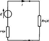
(i) For a purely resistive load and source internal impedance, when X=x=0, maximum power is transferred when R=r
(ii) When the load resistance R and reactance X are both independantly adjustable, maximum power transfer is obtained when X= -x and R=r.
(iii) When the load is purely resistive and adjustable (i.e. X=0), maximum power transfer is obtained when R=|z|, where ![]() .
.
(iv) When the load resistance R is adjustable but reactance X is fixed, maximum power transfer is obtained when ![]() .
.
8. Sometimes networks are complicated and may be transformed using delta-star or star-delta transformations as a preliminary to using a circuit theorem.
Given impedances ZP, ZQ and ZR connected in delta as shown in Figure 15.16(a), then the equivalent in star connection (see Figure 15.16(b)) is given by:

Given impedances Za, Zb and Zc connected in star, as shown Figure 15.16(b), then the equivalent in delta connection Figure 15.16(a) is given by: