1

In parallel circuits, such as those shown in Figure 14.1, the voltage is common to each branch of the network and is thus taken as the reference phasor when drawing phasor diagrams.

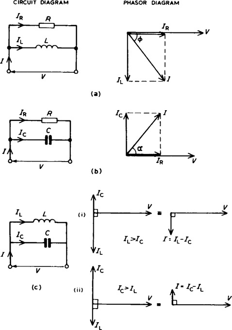
2 R-L parallel circuit

In the two branch parallel circuit containing resistance R and inductance L shown in Figure 14.1(a), the current flowing in the resistance, I_R, is in-phase with the supply voltage V and the current flowing in the inductance, I_L, lags the supply voltage by 90°. The supply current I is the phasor sum of I_R and I_L and thus the current I_L, lags the applied voltage V by an angle lying between 0° and 90° (depending on the values of I_R and I_L), shown as angle ϕ in the phasor diagram.

From the phasor diagram:

$\begin{array}{c}I=\sqrt{\left(I_R^2+I_L^2\right),}(byPythagoras’theorem)\\ where{I}_R=\frac{V}{R}and{I}_L=\frac{V}{X_L}\\ \tan \varphi =\frac{I_L}{I},\sin \varphi =\frac{I_L}{I}and\cos \varphi =\frac{I_R}{I}\end{array}$

(by trigonometric ratios)

$Circuitimpedance,Z=\frac{V}{I}$

3 R-C parallel circuit

In the two branch parallel circuit containing resistance R and capacitance C shown in Figure 14.1(b)), I_R is in-phase with the supply voltage V and the current flowing in the capacitor, I_c, leads V by 90°. The supply current I is the phasor sum of I_R and I_c and thus the current I leads the applied voltage V by an angle lying between 0° and 90° (depending on the values of I_R and I_c), shown as angle a in the phasor diagram.

From the phasor diagram:

$\text{I=}\sqrt{{\text{(I}}_R^2{\text{+ I}}_C^2\text{)}}\text{, (by Pythagoras’ theorem)}$

$\begin{array}{c}where{I}_R=\frac{V}{R}and{I}_C=\frac{V}{X_C}\\ \tan \alpha =\frac{I_C}{I_R},\sin \alpha =\frac{I_C}{I}and\cos \alpha =\frac{I_R}{I}\left(bytrignometricratios\right)\\ CircuitimpedanceZ=\frac{V}{I}\end{array}$

4 L-C parallel circuit

In the two branch parallel circuit containing inductance L and capacitance C shown in Figure 14.1(c),I_L lags V by 90° and I_c leads V by 90°. Theoretically there are three phasor diagrams possible — each depending on the relative values of I_L and I_c.

The latter condition is not possible in practice due to circuit resistance inevitably being present (as in the circuit described in para. 5).

$FortheL-Cparallelcicuit,I_L=\frac{V}{X_L},I_C=\frac{V}{X_C}$

$I=phasordifferencebetween{I}_{L}and{I}_{C}andZ=\frac{V}{I}$

5 LR-C parallel circuit

In the two branch circuit containing capacitance C in parallel with inductance L and resistance R in series (such as a coil) shown in Figure 14.2(a), the phasor diagram for the LR branch alone is shown in Figure 14.2(b) and the phasor diagram for the C branch alone in Figure 14.2(c). Rotating each and superimposing on one another gives the complete phasor diagram shown in Figure 14.2(d).

6

The current I_LR of Figure 14.2(d) may be resolved into horizontal and vertical components. The horizontal component, shown as op is I_LR cos ϕ₁, and the vertical component, shown as pq is I_LR sin ϕ₁. There are three possible conditions for this circuit:

7

There are two methods of finding the phasor sum of currents I_LR and I_C in Figure 14.2(e) and Figure 14.2(f). These are: (i) by a scaled phasor diagram, or (ii) by resolving each current into their ‘in-phase’ (i.e. horizontal) and ‘quadrature’ (i.e. vertical) components.

8

With reference to the phasor diagrams of Figure 14.2:

$\mathrm{Im}pedanceofLRbranch,Z_{LR}=\sqrt{\left(R^2+X_L^2\right)}$

$Current{I}_{LR}=\frac{V}{Z_{LR}}and{I}_C=\frac{V}{X_c}$

$\begin{array}{c}{\text{Supply current I=phasor sum of I}}_{LR}and{I}_C\left(bydrawing\right)\\ =\sqrt{\left\{\left(I_{LR}\cos \varphi \right)+{\left(I_{LR}\sin \varphi \sim I_C\right)}^2\right\}}\left(bycalculation\right)\end{array}$

where ∼ means ’the difference between’.

$CircuitimpedanceZ=\frac{V}{I}$

$\tan {\varphi }_1=\frac{V_L}{V_R}=\frac{X_L}{R},\sin {\varphi }_1=\frac{X_L}{Z_{LR}}and\cos {\varphi }_1=\frac{R}{Z_{LR}}$

$\tan \varphi =\frac{I_{LR}\sin {\varphi }_1\sim I_C}{I_{LR}\cos {\varphi }_1}and\cos \varphi =\frac{I_{LR}\cos {\varphi }_1}{I}$

9

For any parallel ac. circuit:

True or active power, P= VI cos ϕ watts (W) or P=I²_RR watts

Apparent power, S = VI voltamperes (VA)

Reactive power, Q = VI sin ϕ reactive voltamperes (VAr)

$Powerfactor=\frac{truepower}{apparentpower}=\frac{P}{S}=\cos \varphi .$

(These formulae are the same as for series a.c. circuits.)

10

(i) Resonance occurs in the two branch circuit containing capacitance C in parallel with inductance L and resistance R in series (see Figure 14.2(a)) when the quadrature (i.e. vertical) component of current I_LR is equal to I_C. At this condition the supply current I is in-phase with the supply voltage V.

(ii) When the quadrature component ofI_LRis equal to I_C then:

    I_C=I_LR sin ϕ₁(see Figure 14.3)

$Hence\frac{V}{X_C}=\left(\frac{V}{Z_{LR}}\right)\left(\frac{X_L}{Z_{LR}}\right),\left(frompara.8\right)$

    from which,

$Z_{LR}^2=X_C{X}_L=\left(2\pi f_{r}L\right)\left(\frac{1}{\left(2\pi f_{r}C\right)}\right)=\frac{L}{C}$ (1)

(1)

$Hence{\left[\sqrt{\left(R^2+X_L^2\right)}\right]}^2=\frac{L}{C}and{R}^2+X_L^2=\frac{L}{C}$

${\left(2\pi f_{r}L\right)}^2=\frac{L}{C}-R^2$

$f_r=\frac{1}{2\pi L}\sqrt{\left(\frac{L}{C}-R^2\right)}=\frac{1}{2\pi }\sqrt{\left(\frac{L}{L^{2}C}-\frac{R^2}{L^2}\right)}$

    i.e. parallel resonant frequency, f_r, $f_r=\frac{1}{2\pi }\sqrt{\left(\frac{1}{LC}-\frac{R^2}{L^2}\right)}Hz$

    (When R is negligible, then $f_r=\frac{1}{2\pi \sqrt{(LC)}}$ which is the same as for series resonance.)

(iii) Current at resonance,

    I_r =I_LR cos ϕ₁(from Figure 14.3)

$\begin{array}{c}=\left(\frac{V}{Z_{LR}}\right)\left(\frac{R}{Z_{LR}}\right)\left(frompara.8\right)\\ =\frac{VR}{Z_{LR}^2}\end{array}$

    However, frome quation (1), $Z_{LR}^2=\frac{L}{C}$

$Hence{I}_r=\frac{VR}{\left(\frac{L}{C}\right)}=\frac{VRC}{L}$

    The current is at a minimum at resonance.

(iv) Since the current at resonance is in-phase with the voltage the impedance of the circuit acts as a resistance. This resistance is known as the dynamic resistance, R_D (or sometimes, the dynamic impedance).

    From equation (2), impedance at resonance= $\frac{V}{I_r}=\frac{L}{RC}$

    i.e.dynamic resistance, $R_D=\frac{L}{RC}\Omega$.

(v) The parallel resonant circuit is often described as a rejector circuit since it presents its maximum impedance at the resonant frequency and the resultant current is a minimum.

11

Currents higher than the supply current can circulate within the parallel branches of a parallel resonant circuit, the current leaving the capacitor and establishing the magnetic field of the inductor, this then collapsing and recharging the capacitor, and so on. The Q-factor of a parallel resonant circuit is the ratio of the current circulating in the parallel branches of the circuit to the supply current, i.e. the current magnification.

Q-factor at resonance = current magnification

$\begin{array}{c}=\frac{\text{circulating current}}{\text{supply current}}\\ =\frac{I_C}{I_r}=\frac{I_{LR}\sin {\varphi }_1}{I_r}\\ =\frac{I_{LR}\sin {\varphi }_1}{I_{LR}\cos {\varphi }_1}=\frac{\sin {\varphi }_1}{\cos {\varphi }_1}\\ =\tan {\varphi }_1=\frac{X_L}{R}\end{array}$

i.e. Q-factor at resonance $\frac{2\pi f_{r}L}{R}$

(which is the same as for a series circuit).

Note that in a parallel circuit the Q-factor is a measure of current magnification, whereas in a series circuit it is a measure of voltage magnification.

12

At mains frequencies the Q-factor of a parallel circuit is usually low, typically less than 10, but in radio-frequency circuits the Q-factor can be very high.

13

For a particular power supplied, a high power factor reduces the current flowing in a supply system and therefore reduces the cost of cables, switch-gear, transformers and generators. Supply authorities use tariffs which encourage electricity consumers to operate at a reasonably high power factor.

Industrial loads such as a.c. motors are essentially inductive (R-L) and may have a low power factor. One method of improving (or correcting) the power factor of an inductive load is to connect a static capacitor C in parallel with the load (see Figure 14.4(a)). The supply current is reduced from I_LR to I_C, the phasor sum of I_LR and I_C, and the circuit power factor improves from cos ϕ₁ to cos ϕ₂ (see Figure 14.4(b)).

Another example where capacitors are connected directly across a load occurs in fluorescent lighting, where manufacturers include a power-factor correction capacitor inside the fitting.

14

Where a factory possesses a large number of a.c. motors it may be uneconomical to place a capacitor across the terminals of each motor. As the power factor of an individual motor may vary with load, the capacitor may result in overcorrection at certain loads and even produce a voltage surge that may have a damaging effect on the motor. Many factories have automatic power-factor correction plant situated in their substations, capacitors being switched in or out to maintain the system power-factor between certain predetermined limits.