
]>
Appendix 2C: Introduction to the Smith Chart
The Smith chart is a graphical aid or nomogram [1] designed as an aid in radio frequency engineering to assist in solving problems with transmission lines and matching circuits. The reflection coefficient is the relationship based on which the Smith chart is constructed:
The x-axis is the real part of the reflection coefficient (Γr) and the y-axis is the imaginary part of the reflection coefficient (Γi), where
The impedance plotted on the chart will be normalized with respect to the characteristic impedance Z0:
The reflection coefficient can be represented as
and the load impedance as
In polar form, |Γ| and ϕ are, respectively the magnitude and angle of Γ as shown in Figure 2C.1.
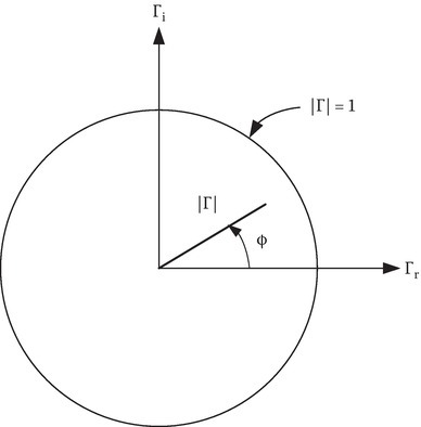
FIGURE 2C.1
Polar coordinates of the Smith chart.
Using Equations 2C.2 and 2C.3, and rearranging to get the real and imaginary parts of zL, it can be seen that
After some further algebraic manipulation, it is found that
Equation 2C.8 represents a family of circles defined by the resistance r. These circles are centered at the point Γr = r/(1 + r), Γi = 0 (which is on the horizontal-axis), and have a radius equal to 1/(1 + r). When r = 0, this is a circle centered at the origin with radius = 1 (the unit circle). On the other hand, if r = ∞, the circle center is at (1, 0) with a radius of zero. Thus, for r = ∞, Equation 2C.8 represents a point on the Γ real axis at the far-right edge of the unit circle. If r = 1, Equation 2C.8 gives a circle centered at (½, 0) with a radius of ½. These circles along with those corresponding to r = ½ and 2 are shown in Figure 2C.2. Note that all the circles are centered on the positive Γr-axis and go through the point Γr = 1 and Γi = 0.
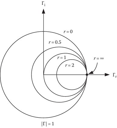
FIGURE 2C.2
Family of circles on the Smith chart corresponding to reflection coefficient for fixed, normalized load resistances.
Equation 2C.9 also represents a family of circles, in this case centered at Γr = 1 and Γi = 1/x with a radius of 1/x. When x = ±∞, this represents a circle centered at (1, 0) with a radius of zero which is again the point at the right edge of the unit circle. If x = 1, the circle is centered at Γ = 1 + j1 with a radius of unity. Since |Γ| is always less than or equal to 1, only the portion of these circles within the unit circle are shown (Figure 2C.2). Figure 2C.3 shows a number of these circular sections for various values of x. Note that the circle representing x = 0 is along the horizontal-axis as the center of the circle moves toward ∞ along the Γr = 1 axis and the radius becomes infinite. As can be seen in Figure 2C.4, both sets of circles are plotted on the Smith chart. If ZL is given, one may divide by Z0 and find the intersection of the appropriate r and x circles and determine Γ from the plot.
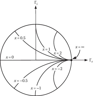
FIGURE 2C.3
Family of circles on the Smith chart corresponding to reflection coefficient for fixed, normalized load reactance.
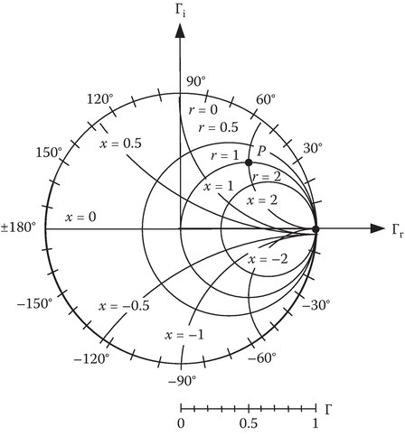
FIGURE 2C.4
Smith chart constant resistance (r) and reactance (x) contours.
To avoid unreadable clutter on the graph, the concentric circles for |Γ| and the radial lines for ϕ are not shown on the Smith chart. But rather graduated line segments at the bottom of the chart and circumference labels of angle around the outer circle are included as shown in Figure 2C.4. As an example, consider the point ZL = 50 + j100 Ω on a 50-Ω line. Then zL = ZL/50 = 1 + j2, so that r = 1 and x = 2. This point is plotted as point P in Figure 2C.4 where it can be seen that |Γ| ≈ 0.7 and ϕ = 45°.
The final scale on the Smith chart, which is used to calculate the distance along a transmission line, is added on the circumference of the plot. The scale is in wavelength units with the zero point taken arbitrarily to the left. It is known that the voltage and the current at any point along a transmission line is given, respectively, by
and
Dividing Equation 2C.10 by Equation 2C.11 and normalizing gives the normalized input impedance:
Replacing z by −d and dividing the numerator and denominator by ejβd, we obtain the general equation relating normalized input impedance, reflection coefficient, and line length (d):
Equation 2C.13 shows that the input impedance at any point z = −d can be obtained by replacing Γ, the reflection coefficient of the load, by Γ e−j2βd. This corresponds to a decrease in the angle of Γ by 2βd radians as we go from the load to the line input. Only the angle of Γ changes, whereas the magnitude stays constant, thus the movement is along a constant radius arc. As we move from the load zL to the input impedance zin, we move toward the generator by a distance d on the transmission line and a clockwise angle 2βd on the Smith chart. One complete rotation around the Smith chart corresponds to a phase change of π radians or when d changes a half wavelength. The Smith chart is thus marked with a scale showing a change of 0.5λ for one circumnavigation of the unit circle. Two scales are normally given, one showing an increase in distance for clockwise movement and the other an increase for counterclockwise rotation. These two scales can be seen on the Smith chart of Figure 2C.5. One scale represents wavelengths toward generator (wtg) and increases for clockwise rotation. The other represents wavelengths toward load (wtl) and increases for counterclockwise rotation.
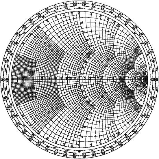
FIGURE 2C.5
The Smith chart (graduated line segments at the bottom are not shown here).
Example 2C.1
The scenario shown in Figure 2C.6 is considered in this example and Figure 2C.7 shows the Smith chart analysis for this example.
Load point A: zL = ZL/Z0 = 2 − j0.5. |Γ| = 0.37, ϕ = −17°. Point A is 0.274 wtg.
Point B, d = 0.6λ, 0.374 wtg
|z(d)|max is at point C and is equal to 2.2 = s (voltage standing wave ratio). This is also the point of voltage maximum. Voltage is maximum when d = [(0.5 − 0.274) + 0.25]λ = 0.476λ.
|z(d)|min is at point D and is equal to 1/2.2 = 0.45. This is also the point of voltage minimum. Voltage is minimum when d = (0.5 − 0.274)λ = 0.226λ.
Point E shows the open-circuit point.
Point F shows the short-circuit point.
Point G shows the point z = 4 + j0.
Point H shows the point z = 0 + j2.
E, F, G, H are not related to the example in Figure 2C.6.

FIGURE 2C.6
Smith chart example (ZL = 100 – j25 Ω, d = 0.6λ).
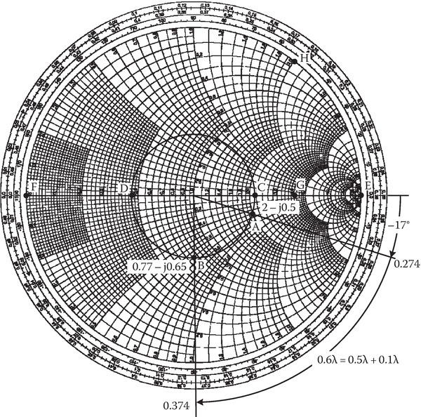
FIGURE 2C.7
Smith chart example A = load 100 – j25Ω, B = input impedance at d = 0.6λ line, C = point of voltage maximum, D = point of voltage minimum, E = open-circuit point, F = short-circuit point, G = load 4 + j0, H = load 0 + j2.
2C.1Reflection of Uniform Plane Waves
Note that the characters with tilde (~) represent a phasor quantity. A superscript plus sign indicates a wave propagating in the +z-direction, whereas a superscript minus sign represents a wave propagating in the −z-direction.
2C.1.1Free Space: Perfect Conductor Interface
Let us consider the following problem depicted in Figure 2C.8.

FIGURE 2C.8
Reflection of uniform plane wave at a free space to perfect conductor boundary.
The space z > 0 is a perfect conductor and the space z < 0 is a free space. A time-harmonic electromagnetic field propagating in the +z-direction in the free space is normally incident on the interface from the left. Let the electric field of this wave be in the x-direction only, that is,
where . The magnetic field of this incident wave is
where The superscript I stands for incident wave. The electric field at z = 0 of this incident wave is . But the boundary condition at z = 0 requires the electric field should be zero. Such a boundary condition can be satisfied if we assume that a reflected wave exists in the free space (propagating in the −z-direction) with the electric and magnetic fields as follows:
and
so
2C.2Comparison with a Transmission Line Problem
A comparison of a normal plane wave reflection (from a free space to a perfect electric conductor) to the transmission line analogy is shown in Figure 2C.9 and summarized in Table 2C.1.

FIGURE 2C.9
Comparison of normal plane wave reflection with transmission line.
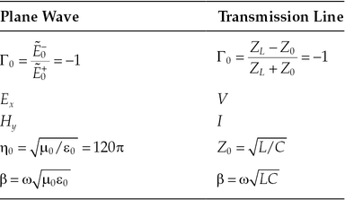
TABLE 2C.1
Plane Wave Reflection Comparison with the Transmission Line Analogy
2C.2.1Dielectric–Dielectric Interface
Let us now consider the problem of reflection of a plane wave at the interface of two dielectrics as depicted in Figure 2C.10.

FIGURE 2C.10
Boundary between two dielectrics.
Let the incident wave be traveling in medium 1 in the positive z-direction and then for z < 0:
Let this give rise to a reflected wave,
and a transmitted wave:
The problem is to determine the reflection coefficient and the transmission coefficient . The boundary conditions give us the required number of equations to solve for Γ0 and T0. The boundary conditions at a dielectric–dielectric interface are continuity of tangential components of and :
or
Using Equations 2C.26 and 2C.28, we obtain
and
2C.3Comparison with a Transmission Line Problem
Figure 2C.11a shows the normal incidence from the left of a plane wave on a dielectric–dielectric interface from dielectric 1 on the left to dielectric 2 on the right. Figure 2C.11b and c shows the transmission line analogy and the equivalent transmission line circuit, respectively. The transmission line 2 extends to infinity. On this line, the wave propagates in the +z-direction and there is no reflected wave. The reflection coefficient at z = ∞ is zero and Γ∞ = 0, and therefore Zin = Z02 (see Figure 2C.11c). The reflection coefficient may now be obtained as follows:
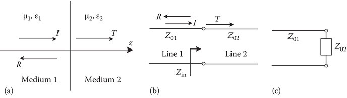
FIGURE 2C.11
Comparison of reflection at a dielectric–dielectric boundary to a transmission line: (a) dielectric interface, (b) transmission line interface, and (c) equivalent load on transmission line.
The purpose of developing the analogy with the transmission lines is to exploit the tools available for transmission line problems for solving the analogous boundary value problems involving plane waves. The Smith chart is one of them. Let us illustrate through a few examples.
Example 2C.2
A 4-GHz uniform plane wave is normally incident from region 1 (z < 0, ε1 = 5, μ1 = 1, σ1 = 0) toward region 2 (z > 0, ε2 = 2, μ2 = 10, σ2 = 0) (Figure 2C.12). Find s (Voltage Standing Wave Ratio) for regions 1 and 2 and the intrinsic impedance (ηin) at z = −0.6 cm.
For region 2, there is no reflected wave, Γ∞ = 0, and s = (1 + Γ)/(1 − Γ) = 1. To determine various quantities in region 1, let us draw an equivalent transmission line (Figure 2C.13). The load is purely resistive and ZL = RL > Z0. Therefore, s in region 1 is ZL/Z0 = 5. To determine ηin at −0.6 cm, we make use of the equivalent transmission line of Figure 2C.14 and the Smith chart shown in Figure 2C.15. In this case,
Load point A is located at r = 5, x = 0 on the Smith chart (0.25 wtg). To reach B on the |Γ| circle, move 0.1789 wtg from A on the |Γ| circle, that is, go to (0.25 + 0.1789) wtg = 0.4289 wtg. From the Smith chart read zB = 0.25 − j0.45. Therefore,
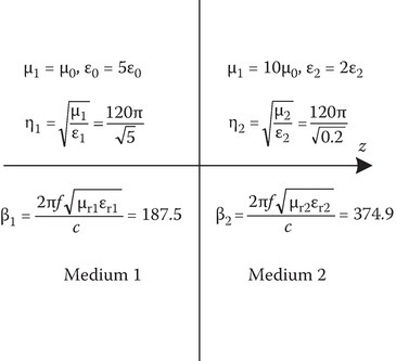
FIGURE 2C.12
Problem geometry for Example 2C.1.
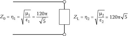
FIGURE 2C.13
Equivalent transmission line circuit for Example 2C.1.

FIGURE 2C.14
Equivalent transmission line circuit with line length d.
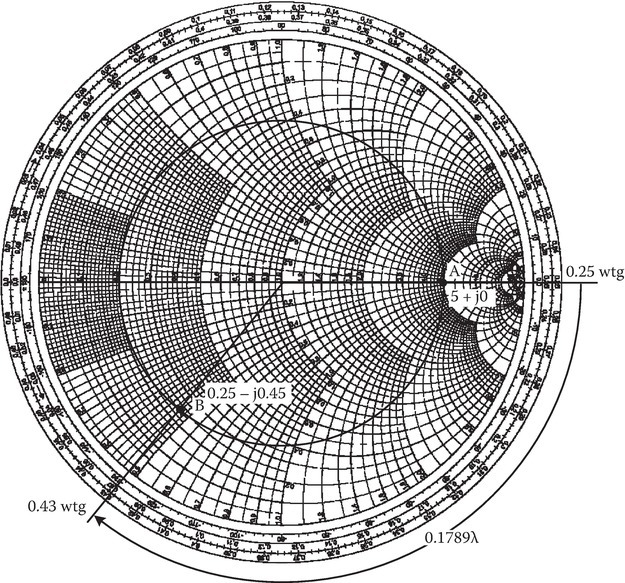
FIGURE 2C.15
Smith chart utilized to solve Example A2.2 dielectric interface problem.
Example 2C.3
Design a radome. A radome is a dielectric material that covers an antenna and protects it from the weather. The thickness of the material should be such that there are no reflections (see Figure 2C.16).
For a transmission line analogy (see Figure 2C.17), it is obvious that ηinput = η0 if d = λ/2. If ηinput = η0, there is a perfect match at interface 1 and there will be no reflections at interface 1.
Consider a numerical example, where a uniform plane wave with λ = 3 cm in the free space is normally incident on a fiberglass (εr = 4.9, σ = 0) radome. (a) What thickness of fiberglass will produce no reflections? (b) What percentage of the incident energy will be transmitted through the fiberglass if the frequency of the incident wave is decreased by 10%?
In this problem, ε1 = 4.9 ε0, f = c/λ = 3 × 10⁸/3 × 10−2 = 10 GHz.
d = λ1/2 = 0.678 cm for no reflections.
If fnew = 0.9f, λ0(new) = c/fnew = λ0/0.9.
Since the physical width d is the same,
Here ηinput may now be obtained by solving the following transmission line problem (Figure 2C.18). To use the Smith chart (Figure 2C.19), let us use normalized values:
But ZL = η0, so This is point A on the Smith chart (r = 2.214, x = 0). Now draw the |Γ| circle and move 0.45 wtg to reach B on the |Γ| circle. Read zB = 1.6 + j0.85.
ηinput = η1 (1.6 + j0.85). The equivalent transmission line load = η1 (1.6 + j0.85)/η0 = 0.723 + j0.384. This normalized load of zL = 0.723 + j0.384 is marked as point C on the Smith chart. To get the reflection coefficient magnitude measure OC = 0.26, |Γ|2 = 0.0676. The transmitted energy = 1 − |Γ|2 = 0.9324 = 93.24%.
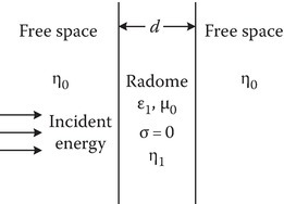
FIGURE 2C.16
Radome analysis geometry.
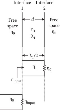
FIGURE 2C.17
Radome equivalent transmission line circuit.
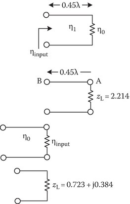
FIGURE 2C.18
Radome equivalent transmission line circuit.
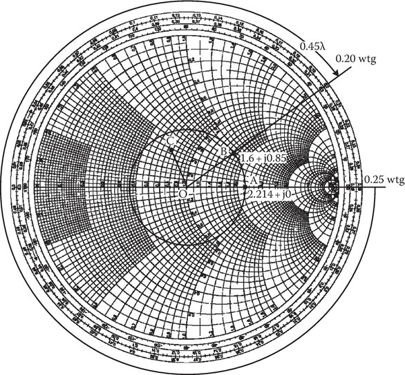
FIGURE 2C.19
Smith chart used in solution of radome problem (Example 2C.1).
2C.4Example of Use of the Smith Chart for Oblique Incidence [2]
The analogy between plane wave reflection problems for oblique incidence and transmission lines is summarized in Table 2C.2.
TABLE 2C.2
A Summary of Plane Wave Reflection (Oblique Incidence) Comparison with the Transmission Line Analogy

Consider the example shown in Figure 2C.20 where we have oblique incidence at an angle of 40° with perpendicular polarization from free space onto two dielectric layers situated within free space at a frequency of 10 GHz.
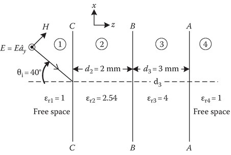
FIGURE 2C.20
Example of use of the Smith chart for oblique incidence.
The incident wave freespace wavelength is
From Snell’s law,
For perpendicular polarization,
The length in wavelengths of each region
and therefore,
Now starting at interface AA, we have the equivalent transmission line shown in Figure 2C.21a that is point A on the Smith chart of Figure 2C.22:
where
Also shown in the Smith chart of Figure 2C.22, moving from point A toward generator 0.189 wavelengths, we read (point B):
and therefore,
which can be seen as point B on the Smith chart and the transmission line of Figure 2C.21b.

FIGURE 2C.21
Equivalent transmission lines for example problem. (a) Transmission line for 3. (b) Transmission line for 2. (c) Renormalization with Z02. (d) Transmission line 1. (e) Renormalization with Z01.

FIGURE 2C.22
Smith chart used in the solution of oblique plane wave reflection from multiple layers.
Renormalizing,
This is represented by point B′ on the Smith chart and the transmission line of Figure 2C.21c. Now moving 0.097 wavelengths toward the generator, we have the transmission line analogy shown in Figure 2C.21d and point C on the Smith chart:
and therefore
Renormalizing, we get
This is represented by point C′ on the Smith chart and the equivalent transmission line of Figure 2C.21e. The reflection coefficient can be read from the Smith chart as
and the power reflection coefficient is given as