
]>
11
Wave in Anisotropic Media and Magnetoplasma*
11.1Introduction
Plasma medium in the presence of a static magnetic field behaves like an anisotropic dielectric. Therefore, the rules of electromagnetic wave propagation are the same as those of the light waves in crystals. Of course, in addition, we have to take into account the dispersive nature of the plasma medium.
The well-established Magnetoionic Theory [1,2,3] is concerned with the study of wave propagation of an arbitrarily polarized plane wave in cold anisotropic plasma, where the direction of phase propagation of the wave is at an arbitrary angle to the direction of the static magnetic field. As the wave travels in such a medium, the polarization state continuously changes. However, there are specific normal modes of propagation in which the state of polarization is unaltered. Waves with the left (L wave) or the right (R wave) circular polarization are the normal modes in the case of phase propagation along the static magnetic field. Such propagation is labeled as longitudinal propagation. Ordinary wave (O wave) and the extraordinary wave (X wave) are the normal modes for transverse propagation. The properties of these waves are explored in Section 11.3, Section 11.4 and Section 11.5.
11.2Basic Field Equations for a Cold Anisotropic Plasma Medium
In the presence of a static magnetic field B0, the force equation needs modification due to the additional magnetic force term:
The corresponding modification of the constitutive relation in terms of J is given by
where
In the above, ˆB0
Equations 1.1 and 1.2 are repeated here for convenience:
and Equation 11.2 is the basic equation that will be used in discussing the electromagnetic wave transformation by magnetized cold plasma.
Taking the curl of Equation 11.4 and eliminating H, the wave equation for E can be derived:
Similar efforts will lead to a wave equation for the magnetic field:
where
If ω2p
Equations 11.6 and 11.7 involve more than one field variable. It is possible to convert them into higher-order equations in one variable. In any case, it is difficult to obtain meaningful analytical solutions to these higher-order vector partial differential equations. The equations in this section are useful in developing numerical methods.
We will consider next, as in the isotropic case, simple solutions to particular cases where we highlight one parameter or one aspect at a time. These solutions will serve as building blocks for the more involved problems.
11.3One-Dimensional Equations: Longitudinal Propagation and L and R Waves
Let us consider the particular case where (1) the variables are functions of one spatial coordinate only, say the z-coordinate, (2) the electric field is circularly polarized, (3) the static magnetic field is z-directed, and (4) the variables are denoted by
The basic equations for E, H, and J take the following simple form:
If ωp and ωb are functions of time only, then Equation 11.19 reduces to
Let us next look for the plane wave solutions in a homogeneous, time-invariant unbounded magnetoplasma medium, that is,
where f stands for any of the field variables E, H, or J. From Equations 11.16 and 11.17, it is shown that
where
This shows clearly that the magnetized plasma, in this case, can be modeled as a dielectric with the dielectric constant given by Equation 11.25. The dispersion relation is obtained from
which when expanded gives
The expression for the dielectric constant can be written in an alternate fashion in terms of ωc1 and ωc2 which are called cutoff frequencies: the dispersion relation can also be recast in terms of the cutoff frequencies as
In the above, the top sign is for the right circular polarization (R wave) and the bottom sign is for the left circular polarization. Figure 11.1 gives εp versus ω and Figure 11.2 the ω−k diagram, respectively, for the R wave. Figures 11.3 and 11.4 do the same for the L wave. R and L waves propagate in the direction of the static magnetic field, without any change in the polarization state of the wave and are called the characteristic waves of longitudinal propagation. For these waves, the medium behaves like an isotropic plasma except that the dielectric constant εp is influenced by the strength of the static magnetic field. Particular attention is drawn to Figure 11.1 which shows that the dielectric constant εp > 1 for the R wave in the frequency band 0 < ω < ωb. This mode of propagation is called whistler mode in the literature on ionospheric physics and helicon mode in the literature on solid-state plasma. Note that an isotropic plasma does not support a whistler wave.

FIGURE 11.1
Dielectric constant for an R wave.

FIGURE 11.2
ω–k diagram for an R wave.
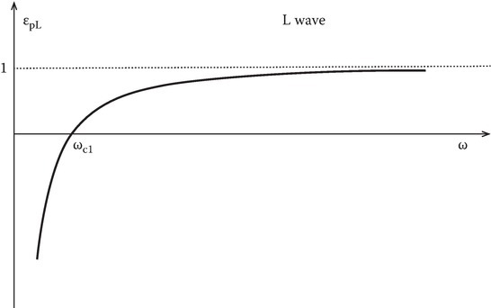
FIGURE 11.3
Dielectric constant for an L wave.
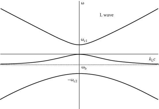
FIGURE 11.4
ω–k diagram for an L wave.
The longitudinal propagation of a linearly polarized wave is accompanied by the Faraday rotation of the plane of polarization. This phenomenon is easily explained in terms of the propagation of the R and L characteristic waves. A linearly polarized wave is the superposition of R and L waves each of which propagates without change of its polarization state but each with a different phase velocity. (Note from Equation 11.25 that εp for a given ω, ωp, and ωb is different for R and L waves due to the sign difference in the denominator.) The result of combining the two waves, after traveling a distance d, is a linearly polarized wave again but with the plane of polarization rotated by an angle ψ given by
Appendix 11A discusses Faraday rotation in more detail.
The high value of εp in the lower-frequency part of the whistler mode can be demonstrated by the following calculation given in [2]; for fp = 1014 Hz, fb = 1010 Hz, and f = 10 Hz, εp = 9 × 10¹⁶. The wavelength of the signal in the plasma is only 10 cm. See [4,5,6] for literature on the associated phenomena.
The resonance of the R wave at ω = ωb is of special significance. Around this frequency, it can be shown that even a low-loss plasma strongly absorbs the energy of a source electromagnetic wave and heats the plasma. This effect is the basis of radio frequency heating of Fusion Plasmas [7]. It is also used to experimentally determine the effective mass of an electron in a crystal [8].
For the L wave, Figure 11.3 does not show any resonance effect. In fact, the L wave has resonance at the ion gyrofrequency. In the Lorentz plasma model, the ion motion is neglected. A simple modification, by including the ion equation of motion, will extend the EMW transformation theory to a low-frequency source wave [2,9,10,11].
11.4One-Dimensional Equations: Transverse Propagation—O Wave
Let us next consider that the electric field is linearly polarized in the y-direction, that is,
The last term on the RHS of Equation 11.2 is zero since the current density and the static magnetic field are in the same direction. The equations then are no different from those of the isotropic case and the static magnetic field has no effect. The electrons move in the direction of the electric field and give rise to a current density in the plasma in the same direction as that of the static magnetic field. In such a case, the electrons do not experience any magnetic force and their orbit is not bent and they continue to move in the direction of the electric field. The one-dimensional solution for a plane wave in such a medium is called an ordinary wave or O wave. Its characteristics are the same as those discussed in the previous chapters. In this case, unlike the case considered in Section 11.2, the direction of phase propagation is perpendicular to the direction of the static magnetic field and hence this case comes under the label of transverse propagation.
11.5One-Dimensional Solution: Transverse Propagation—X Wave
The more difficult case of the transverse propagation is when the electric field is normal to the static magnetic field. The trajectories of the electrons that start moving in the direction of the electric field get altered and bent due to the magnetic force. Such a motion gives rise to an additional component of the current density in the direction of phase propagation and to obtain a self-consistent solution we have to assume that a component of the electric field exists also in the direction of phase propagation. Let
The basic equations for E, H, and J take the following form:
Let us look again for the plane wave solution in a homogeneous, time-invariant, unbounded magnetoplasma medium by applying Equation 11.21 to set Equation 11.42, Equation 11.43, Equation 11.44, Equation 11.45, Equation 11.46:
From Equation 11.49, Equation 11.50, Equation 11.51, we get the following relation between Jx and Ex:
Substituting Equation 11.52 into Equation 11.48,
An alternate expression for εpX can be written in terms of ωc1, ωc2, and ωuh:
The cutoff frequencies ωc1 and ωc2 are defined earlier and ωuh is the upper hybrid frequency:
The dispersion relation k2 = (ω2/c2)εpX, when expanded, gives
In obtaining Equation 11.57, the expression for εpX given by Equation 11.54 is used. For the purpose of sketching the ω–k diagram, it is more convenient to use Equation 11.54 for εpX and write the dispersion relation as
Figures 11.5 and 11.6 sketch εpX versus ω, and ω versus kc, respectively. Substituting Equations 11.49 and 11.52 into Equation 11.51, we can find the ratio of Ez to Ex:
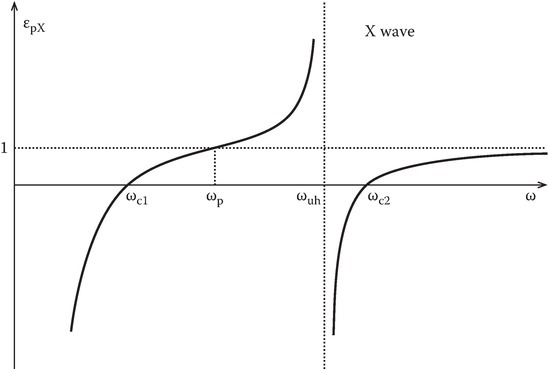
FIGURE 11.5
Dielectric constant for an X wave.
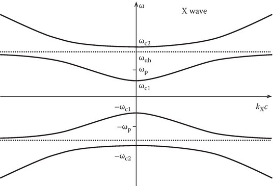
FIGURE 11.6
ω–k diagram for an X wave.
This shows that the polarization in the x–z-plane, whether linear, circular, or elliptic, depends on the source frequency and the plasma parameters. Moreover, using Equations 11.52 and 11.49, the relation between J and E can be written as
where ˉs
where the dielectric tensor ˉK
which gives, for this case,
This shows that Dz = 0, even when Ez ≠ 0. For the X wave, D, H, and the direction of propagation are mutually orthogonal. While E and H are orthogonal, E and ˆk
In the above, npX is the refractive index. Figure 11.7 is a geometrical sketch of the directions of various components of the X wave. The direction of the power flow is given by the Poynting vector S = E × H which, in this case, is not in the direction of phase propagation. The result that Dz = 0 for the plane wave comes from the general equation
in a sourceless medium. In an anisotropic medium, it does not necessarily follow that the divergence of the electric field is also zero because of the tensorial nature of the constitutive relation. For example, from the expression
Dz can be zero without Ez being zero.
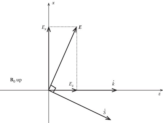
FIGURE 11.7
Geometrical sketch of the directions of various components of the X wave.
11.6Dielectric Tensor of a Lossy Magnetoplasma Medium
The constitutive relation for a lossy plasma with collision frequency ν (rad/s) is obtained by modifying Equation 11.2 further:
Assuming time-harmonic variation exp(jωt) and taking the z-axis as the direction of the static magnetic field,
we can write Equation 11.70 as
and
Equation 11.72 can be written as
Combining Equation 11.75 with (11.73), we obtain
where
In the above, σ⊥, σH, and σ∣∣ are called perpendicular conductivity, Hall conductivity, and parallel conductivity, respectively. From Equation 11.63, the dielectric tensor ˉK can now be obtained:
where
11.7Periodic Layers of Magnetoplasma
Layered semiconductor–dielectric periodic structures in dc magnetic field can be modeled as periodic layers of magnetoplasma. Electromagnetic wave propagating in such structures can be investigated by using the dielectric tensor derived in Section 11.6. The solution is obtained by extending the theory of Section 9.7 to the case where the plasma layer is magnetized and hence has the anisotropy complexity [12]. Brazis and Safonova [13,14,15] investigated the resonance and absorption bands of such structures.
11.8Surface Magnetoplasmons
The theory of Section 9.8 can be extended to the propagation of surface waves at a semiconductor–dielectric interface in the presence of a static magnetic field. The semiconductor in a dc magnetic can be modeled as an anisotropic dielectric tensor. Wallis [16] discussed at length the properties of surface magnetoplasmons on semiconductors.
11.9Surface Magnetoplasmons in Periodic Media
Wallis et al. [17,18] discuss the propagation of surface magnetoplasmons in truncated superlattices. This model is a combination of the models used in Sections 11.7 and 11.8.
11.10Permeability Tensor
Ferrite material (see Section 8.9) in the presence of a static magnetic field behaves like an anisotropic magnetic media. The wave propagation in such a medium has properties similar to the magnetoplasma. The permeability is a tensor. Appendix 11B discusses the permeability tensor.
11.11Reflection by a Warm Magnetoplasma Slab
We discussed the slab problem in the case of a cold plasma slab in Section 9.4 and a warm plasma slab in Appendix 10A. The more general problem is that of a warm magnetoplasma slab. The essence of this problem can be understood by considering the normal incidence involving the coupling of an electromagnetic wave with an electron plasma wave, as shown in Appendix 11C.
References
- 1.Heald, M.A. and Wharton, C. B., Plasma Diagnostics with Microwaves, Wiley, New York, 1965.
- 2.Booker, H.G., Cold Plasma Waves, Kluwer Academic Publishers, Hingham, MA, 1984.
- 3.Swanson, D.G., Plasma Waves, Academic Press, New York, 1989.
- 4.Steele, M.C., Wave Interactions in Solid State Plasmas, McGraw-Hill, New York, 1969.
- 5.Bowers, R., Legendy, C., and Rose, F., Oscillatory galvanometric effect in metallic sodium, Phys.Rev. Lett., 7, 339, 1961.
- 6.Aigrain, P.R., Proceedings of the International Conference on Semiconductor Physics, Czechoslovak Academy Sciences, Prague, Czech Republic, p. 224, 1961.
- 7.Miyamoto, K., Plasma Physics for Nuclear Fusion, The MIT Press, Cambridge, MA, 1976.
- 8.Solymar, L. and Walsh, D., Lectures on the Electrical Properties of Materials, 5th edn., Oxford University Press, Oxford, U.K., 1993.
- 9.Madala, S.R.V. and Kalluri, D.K., Longitudinal propagation of low frequency waves in a switched magnetoplasma medium, Radio Sci., 28, 121, 1993.
- 10.Dimitrijevic, M.M. and Stanic, B. V., EMW transformation in suddenly created two-component magnetized plasma, IEEE Trans. Plasma Sci., 23, 422, 1995.
- 11.Madala, S.R. V., Frequency shifting of low frequency electromagnetic waves using magnetoplasmas, Doctoral thesis, University of Massachusetts Lowell, Lowell, MA, 1993.
- 12.Kalluri, D.K., Electromagnetics of Time Varying Complex Media: Frequency and Polarization Transformer, CRC Press/Taylor & Francis Group, Boca Raton, FL, 2010.
- 13.Brazis, R.S. and Safonova, L. S., Resonance and absorption band in the classical magnetoactive semiconductor–insulator superlattice, Int. J. Infrared Millim. Waves, 8, 449, 1987.
- 14.Brazis, R.S. and Safonova, L. S., Electromagnetic waves in layered semiconductor–dielectric periodic structures in DC magnetic fields, Proc. SPIE, 1029, 74, 1988.
- 15.Brazis, R.S. and Safonova, L. S., In-plane propagation of millimeter waves in periodic magnetoactive semiconductor structures, Int. J. Infrared Millim. Waves, 18, 1575, 1997.
- 16.Wallis, R.F., Surface magnetoplasmons on semiconductors, in: Boardman, A. D. (Ed.), Electromagnetic Surface Modes, Wiley, New York, 1982, Chap. 2.
- 17.Wallis, R.F., Szenics, R., Quihw, J. J., and Giuliani, G. F., Theory of surface magnetoplasmon polaritons in truncated superlattices, Phys. Rev. B, 36, 1218, 1987.
- 18.Wallis, R.F. and Quinn, J. J., Surface magnetoplasmon polaritons in truncated superlattices, Phys. Rev. B, 38, 4205, 1988.