
]>
1
Electromagnetics of Simple Media*
1.1Introduction
The classical electromagnetic phenomena are consistently described by Maxwell’s equations; these vector (see Appendix 1A) equations in the form of partial differential equations are
where, in standard (RMKS) units, E is the electric field intensity (V/m), H the magnetic fieldintensity (A/m), D the electric flux density (C/m2), B the magnetic flux density (Wb/m2), J the volume electric current density (A/m2), and ρV the volume electric charge density (C/m3).
In the above equation, J includes the source current Jsource.
The continuity equation
and the force equation on a point charge q moving with a velocity ν
are often stated explicitly to aid the solution of problems. In the above equation, q is the charge (C) and ν the velocity (m/s).
Solutions of difficult electromagnetic problems are facilitated through the definitions of electromagnetic potentials (see Appendix 1B):
where A is the magnetic vector potential (Wb/m) and Φ the electric scalar potential (V).
The effect of an electromagnetic material on the electromagnetic fields is incorporated in constitutive relations between the fields E, D, B, H, and J.
1.2Simple Medium
A simple medium has the constitutive relations
where ε0 and μ0 are the permittivity and permeability of the free space, respectively,
Different materials have different values for the relative permittivity εr (also called the dielectric constant), the relative permeability μr, and the conductivity σ (S/m). A simple medium further assumes εr, μr, and σ to be positive scalar constants (see Figure 1.1).
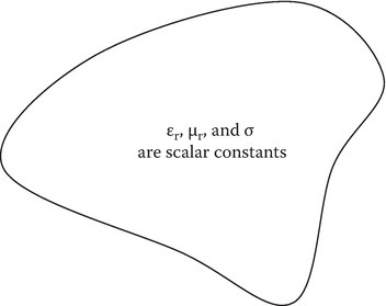
FIGURE 1.1
Idealization of a material as a simple medium.
Such an idealization of material behavior is possible in the solution of some electromagnetic problems in certain frequency bands. In fact, the first course in electromagnetics often deals with such problems only. In spite of such an idealization, the electromagnetic problems may still need the use of heavy mathematics for analytical solutions due to the size, shape, and composition of the materials in a given volume of space. At a spatial interface between two materials, the fields on the two sides of the boundary can be related through boundary conditions (Figure 1.2):
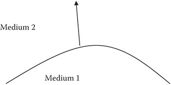
FIGURE 1.2
Boundary conditions.
In the above, ρs is the surface charge density (C/m2), K is the surface current density (A/m), and ˆn12
1.3Time-Domain Electromagnetics
The equations developed so far are the basis for determining the time-domain electromagnetic fields in a simple medium. For a lossless (σ = 0) simple medium, the solution is often obtained by solving for potentials A and Φ, which satisfy the simple form of wave equations
where
In obtaining the above equations, we used the Lorentz condition
The terms on the right-hand sides of Equations 1.18 and 1.19 are the sources of the electromagnetic fields. If they are known, Equations 1.18 and 1.19 can be solved using the concept of retarded potentials:
where the symbols in square brackets are the values at a retarded time, that is,
and r and r′ are the position vectors describing the field point and the source point, respectively (see Figure 1.3a). After solving for A and Φ, the electromagnetic fields are obtained by using Equations 1.7 and 1.8. We can then obtain the power density S (W/m2) on the surface s:
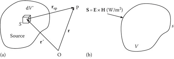
FIGURE 1.3
(a) Source point and field point. (b) Poynting theorem.
The interpretation that S is the instantaneous power density follows from the Poynting theorem (see Appendix 1C) applied to a volume V bounded by a closed surface s (Figure 1.3b):
Equation 1.27 is obtained from Equations 1.1 and 1.2 and is the mathematical statement of conservation of energy.
1.3.1Radiation by an Impulse Current Source
The computation of the time-domain electric and magnetic fields radiated into free space due to a time-varying current is illustrated through a simple example. Let the source be an impulse current in a small piece of wire of very small length h. The source can be modeled as a point dipole with
where δ(t) is an impulse function defined by
The geometry is shown in Figure 1.4.

FIGURE 1.4
Impulse current source modeled as a point dipole for very small length h.
Since the source is a filament, Equation 1.22 becomes
and
Since h is very small, we can approximate rsp by r and from Equation 1.29:
Expressing the unit vector ˆz in spherical coordinates, we obtain
the vector potential in spherical coordinates is given by
The time-domain magnetic field H is given by
From Equations 1.32 and 1.33, evaluating curl in spherical coordinates, we obtain
The electric field E can be computed from the Maxwell equation
Such an evaluation gives EΦ = 0 and
In the above, u(t) is a Heaviside step function defined by
The problem has the following physical significance. The impulse current creates at t = 0, a dipole as shown in Figure 1.5. Two charges initially at the same location are suddenly separated by a small distance h. Noting that (d[u(t)])/dt = δ(t), q in Figure 1.5 is equal to I0. Equations 1.34 and 1.36 show that the fields are zero until the instant t = r/c at which the wave front reaches the observation point. At that instant the fields are discontinuous but immediately after that instant, the magnetic field is zero and the electric field has a value corresponding to a static electric dipole of dipole moment
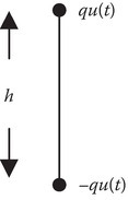
FIGURE 1.5
The impulse current source and its equivalent electric point dipole.
1.4Time-Harmonic Fields
A particular case of time-domain electromagnetics is time-harmonic electromagnetics where we assume that the time variations are harmonic (cosinusoidal). The particular case is analogous to steady-state analysis in circuits and makes use of phasor concepts. A field component is expressed as
where ˜F(r) is the phasor–vector field. The special symbol ~ denotes a phasor distinct from the real-time harmonic field and will be used where it is necessary to make such a distinction. When there is no likelihood of confusion the special symbol will be dropped, the phasor and the real-time harmonic field will be denoted in the same way, and the meaning of the symbol will be understood from the context. Consequently, the time-domain fields are transformed to phasor fields by noting that partial differentiation with respect to time in time-domain transforms as multiplication by jω in the phasor (frequency) domain. Hence, the phasor form of the fields satisfies the following equations:
In the above
〈SR〉 is the time-averaged real power density, the symbol * denotes complex conjugate, and k is the wave number. Several remarks are in order. The program of analytical computation of phasor fields given by the harmonic sources is easier than the corresponding computation of time-domain fields indicated in the last section. We can compute Ã(r) from Equation 1.50 and obtain ˜Φ(r) in terms of à from Equation 1.49. The time-harmonic electric and magnetic fields are then computed using Equations 1.45 and 1.46. The second remark concerns the boundary conditions. For the time harmonic case, only two of the four boundary conditions given in Equation 1.14, Equation 1.15, Equation 1.16 and Equation 1.17 are independent.
1.5Quasistatic and Static Approximations
Quasistatic approximations are obtained by neglecting either the magnetic induction or the displacement current. The former is electrostatic and the latter is magnetostatic. Maxwell’s Equation 1.1, Equation 1.2, Equation 1.3 and Equation 1.4 take the following forms.
Electroquasistatic:
(1.54a)∇×E=0,(1.55a)∇×H=J+∂D∂t,(1.56a)∇⋅D=ρV,(1.57a)∇⋅B=0.Magnetoquasistatic:
(1.54b)∇×E=−∂B∂t,(1.55b)∇×H=J,(1.56b)∇⋅D=ρV,(1.57b)∇⋅B=0.
If both the time derivatives are neglected in Maxwell equations, they decompose into two uncoupled sets describing electrostatics and magnetostatics.
Electrostatics:
(1.58a)∇×E=0,(1.59a)∇⋅D=ρVMagnetostatics:
(1.58b)∇×H=J,(1.59b)∇⋅B=0.
A quantitative discussion of these approximations is given in Appendix 1D, based on a time-rate parameter.
1.6Maxwell’s Equations in Integral Form and Circuit Parameters
Equation 1.1, Equation 1.2, Equation 1.3 and Equation 1.4 are partial differential equations. When Equations 1.1 and 1.2 are integrated over an open surface bounded by a closed curve, and Stokes’ theorem (1A.66) is used, we get the first two integral forms of the Maxwell’s equations. When Equations 1.3 and 1.4 are integrated over a definite volume bounded by a closed surface, and divergence theorem (1A.67) is used, we get the last two of the Maxwell’s equations in the integral form. Lumped-parameter circuit theory is a low-frequency approximation of the integral form of the first two Maxwell’s equations. One must make a quantitative check of the validity of the low-frequency approximation before applying the circuit theory to the electromagnetic field problems. Some details of the integral forms and circuit concepts derived from them are given next.
Equation 1.1 relates the E field at a point with B field at the same point. When integrated over an open surface bounded by a closed curve and with the application of (1A.66), it will lead to
where c is a closed curve bounding the open surface s. In Equation 1.60, if the surface s is moving, that is, s = s(t) and c = c(t), E and B in Equation 1.60 are those measured by an observer, who is at rest with respect to the moving media. If E and B are measured by an observer at rest in the laboratory, Equation 1.60 takes the form [1,2]
In the above
term1: total induced voltage
term2: total time rate of decrease of the magnetic flux Φm
term3: transformer part of the induced voltage
term4: motional part of the induced voltage, where v is the velocity of c(t)
Additional discussion from the view point of moving media can be found in Sections 14.3 and 14.4
When the deformation of the moving circuit c(t) is continuous, the total induced voltage is easier to compute by evaluating term2 than evaluating term3 and term4 separately and adding them.
The concept of the circuit element inductance L and its volt–ampere (V–I) relationship
can be obtained from Equation 1.61. Let us define inductance L in henries (abbreviated as H) as the magnetic flux Φm generated by a current I, that is
From Equation 1.61 and noting the induced voltage (also referred to as emf) is opposite in sign to the voltage drop V,
In multiturn systems or situations where all the flux is not external to the current that generates it (e.g., the magnetic flux in a conductor due to the current flowing in the conductor), the concept of flux linkages is used [3].
Next, we will develop the second Maxwell’s equation in integral form and use it to explain the capacitance circuit parameter and the concept of displacement current. Equation 1.2 can also be transformed to integral form, using Stokes’ theorem again (1A.66):
where, again, the closed curve c is the bound for an open surface s. From Figure 1.6, it is clear that s is not unique. The closed curve c is the bound for all the open surfaces s1, s2, and s3, the implication of which will be used to explain a current jumping through a perfect dielectric in a capacitor. Let us state in words the meaning of various terms marked in Equation 1.65:
term1: circulation of H field over c
term2: conduction current IC in amperes
term3: displacement current ID in amperes.
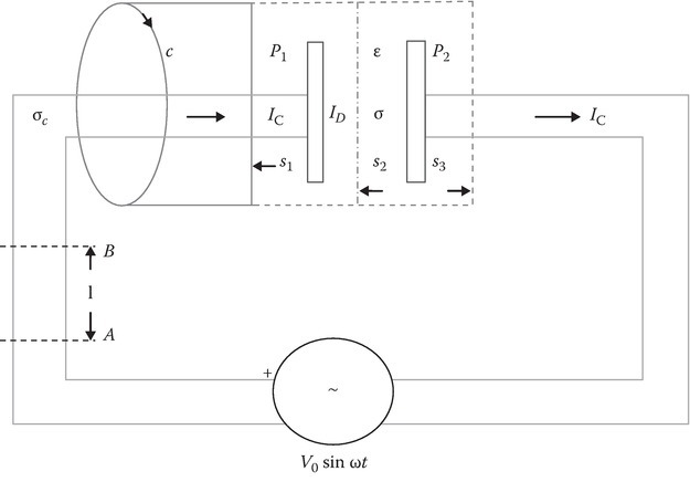
FIGURE 1.6
Integral form of Maxwell–Ampere law (Equation 1.65): Explanation of circuit elements and displacement current.
The capacitance circuit parameter C is defined as
where Q is the magnitude of the charge on either of the two perfect conductors embedded in a perfect dielectric medium and V is the potential difference between the two conductors. The V–I relationship of a two terminal capacitive circuit element is given by
If we identify this current as ID (term3) in Equation 1.65
Thus, we can write
With reference to Figure 1.6, if E is in the z direction, independent of the coordinates, and ε is a constant
where A is the plate area.
Suppose the dielectric is a low-loss medium with a small conductivity σ, as shown in Figure 1.6; one can define the conductance G as
For uniform E and constant σ
The parallel plate capacitor with a low-loss dielectric shown in Figure 1.6 can be modeled as C given by Equation 1.70 in parallel with G given by Equation 1.72.
Suppose the connecting wires in Figure 1.6 are not perfect but are good conductors of conductivity σc. The familiar form of Ohm’s law is
where RAB is the resistance of the conductor between the planes A and B:
For the case of constant J and σc
where S is the cross-sectional area of the wire. For the current flow governed by the skin effect, S is not the physical cross-sectional area but an effective cross-sectional area. Section 2.6 discusses this case.
Maxwell called term3 as displacement current. Let us explore its role in explaining the flow of the same conduction current through the wires attached to the two plates P1 and P2. Let us assume the ideal situation of σ = 0 and σc = infinity. The conduction current flowing through the wires is given by
The displacement current in the wires is very small compared to IC. This is term2, where the surface s is either s1 or s3 in Figure 1.6. Without the concept of the displacement current, it is difficult to explain the jumping of the current from the left wire to the right wire since the dielectric in the capacitor is a perfect insulator (σ = 0). However, we show below that the ID given by term3 in Equation 1.65 will be exactly the same as IC:
The integral form of Equation 1.3 is obtained by integrating over a definite volume v bounded by a closed surface s:
In the above, we used divergence theorem (1A.67). The word statement for Equation 1.78 is that the electric flux coming out of a closed surface is the net positive charge enclosed by the surface (Gauss’s law).
Similar operations on Equation 1.4 give
leading to the word statement that the magnetic flux coming out of a closed surface is zero. The magnetic flux lines close on themselves, thus ruling out the existence of magnetic monopoles. The familiar source of a small loop of current for magnetic fields can be shown to be equivalent to a magnetic dipole. This aspect is discussed in Section 8.9.
Integration of Equation 1.5 over a fixed surface leads to the mathematical statement of the principle of conservation of charge:
The first term in Equation 1.80 is the current going out of the fixed closed surface s and the last term is the time rate of decrease of the charge in the volume v.
References
- 1.Kalluri, D.K., Electromagnetic Waves, Materials, and Computation with MATLAB, 2nd edn., CRC Press, Taylor & Francis Group, Boca Raton, FL, 2016.
- 2.Rothwell, J.R. and Cloud, M. J., Electromagnetics, CRC Press, Taylor & Francis Group, Boca Raton, FL, 2001.
- 3.Hayt, Jr., W.H., Engineering Electromagnetics, 5th edn., McGraw-Hill, New York, 1989.