
]>
9
Waves in Isotropic Cold Plasma: Dispersive Medium*
In Section 8.4, we briefly discussed the plasma medium and characterized it by the associated parameter called the plasma frequency ωp, which is related to the electron density N through Equation 8.22. In Chapter 10, we will discuss quantitatively the various technical terms used in describing the plasma state of matter.
In this chapter, we consider the wave propagation in an isotropic cold (thermal effects neglected) plasma medium. We start with the equation for the force experienced by the electron in the plasma medium due to the wave electric and magnetic fields, given by
It can be shown that the force due to the wave magnetic field is negligible compared to the force due to the wave electric field.
The plasma current density J is related to its density N by
After neglecting the ν × B term in (9.1a), and using (8.22) and (9.1b), one can obtain the equation relating J and E:
Let us assume that the electron density varies only in space (inhomogeneous isotropic plasma):
9.1Basic Equations
One can then construct basic solutions by assuming that the field variables vary harmonically in time:
In the above, F(r) stands for any of E, H, or J phasors. The basic field equations are then given by
Combining Equations 9.4 and 9.5, we can write
where εp is the dielectric constant of the isotropic plasma and is given by
The vector wave equations are
The scalar one-dimensional equations take the form
Combining Equations 9.11 and 9.12, or from Equations 9.6, we have
where
Figure 9.1 shows the variation of εp with ω. εp is negative for ω < ωp, 0 for ω = ωp, and positive but less than 1 for ω > ωp. The scalar one-dimensional wave equations, in this case, reduce to Equations 9.15 and 9.16:
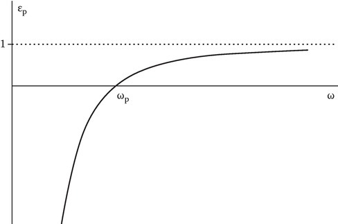
FIGURE 9.1
Dielectric constant versus frequency for a plasma medium.
Equation 9.15 can easily be solved if we further assume that the dielectric is homogeneous (εp is not a function of z). Such a solution is given by
where
Here, n is the refractive index and k0 is the free-space wave number. The first term on the RHS of Equation 9.17 represents a traveling wave in the positive z-direction (positive-going wave) of angular frequency ω and wave number k and the second term a similar but negative-going wave. The z-direction is the direction of phase propagation, and the velocity of phase propagation vp (phase velocity) of either of the waves is given by
From Equation 9.10,
where
Here η is the intrinsic impedance of the medium. The waves described above which are one-dimensional solutions of the wave equation in an unbounded isotropic homogeneous medium are called uniform plane waves in the sense that the phase and the amplitude of the waves are constant in a plane. Such one-dimensional solutions in a coordinate-free description are called transverse electric and magnetic waves (TEM) and for an arbitrarily directed wave their properties can be summarized as follows:
In the above, ˆk is a unit vector in the direction of phase propagation. In other words, the properties are:
Unit electric field vector, unit magnetic field vector, and the unit vector in the direction of (phase) propagation form a mutually orthogonal system.
There is no component of the electric or the magnetic field vector in the direction of propagation.
The ratio of the electric field amplitude to the magnetic field amplitude is given by the intrinsic impedance of the medium.
Figure 9.2 shows the variation of the dielectric constant εp with frequency for a typical real dielectric. For such a medium, in a broad frequency band, εp can be treated as not varying with ω and denoted by the dielectric constant εr. We will next consider the step profile approximation for a dielectric profile. In each of the media 1 and 2, the dielectric can be treated as homogeneous. The solution for this problem is well known but is included here to provide a comparison with the solutions in Chapter 10, Chapter 11 and Chapter 12.
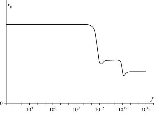
FIGURE 9.2
Sketch of the dielectric constant of a typical material.
9.2Dielectric–Dielectric Spatial Boundary
The geometry of the problem is shown in Figure 9.3. Let the incident wave in medium 1, also called the source wave, have the fields
where ωi is the frequency of the incident wave and

FIGURE 9.3
Dielectric–dielectric spatial boundary problem.
The fields of the reflected wave are given by
where ωr is the frequency of the reflected wave and
The fields of the transmitted wave are given by
where ωr is the frequency of the transmitted wave and
The boundary condition of the continuity of the tangential component of the electric field at the interface z = 0 can be stated as
The above must be true for all x, y, and t. Thus, we have
Since Equation 9.38 must be satisfied for all t, the coefficients of t in the exponents of Equation 9.38 must match:
The above result can be stated as follows: the frequency ω is conserved across a spatial discontinuity in the properties of an electromagnetic medium. As the wave crosses from one medium to the other in space, the wave number k changes as dictated by the change in the phase velocity (see Figure 9.4).
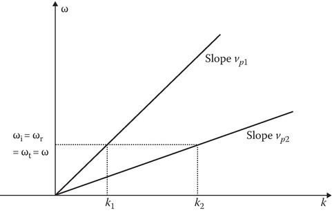
FIGURE 9.4
Conservation of frequency across a spatial boundary.
From Equations 9.38 and 9.39, we obtain
The second independent boundary condition of continuity of the tangential magnetic field component is written as
The reflection coefficient RA = Er/E0 and the transmission coefficient TA = Et/E0 are determined using Equations 9.40 and 9.41. From Equation 9.41, we have
The results are as follows:
The significance of the subscript A in the above is to distinguish from the reflection and transmission coefficients due to a temporal discontinuity in the properties of the medium.
We next show that the time-averaged power density of the source wave is equal to the sum of the time-averaged power density of the reflected and the transmitted waves:
The LHS is
whereas the RHS is
9.3Reflection by a Plasma Half-Space
Let an incident wave of frequency ω traveling in the free space (z < 0) be incident normally on the plasma half-space (z > 0) of plasma frequency ωp. The intrinsic impedance of the plasma medium is given by
From Equation 9.43, the reflection coefficient RA is given by
where
is the source frequency normalized with respect to the plasma frequency. The power reflection coefficient ρ = |RA|2 and the power transmission coefficient τ (=1 − ρ) versus Ω are shown in Figure 9.5. In the frequency band 0 < ω < ωp, the characteristic impedance ηp is imaginary. The electric field EP and the magnetic field HP in the plasma are in time quadrature; the real part of (EP×H*P) is zero. The wave in plasma is an evanescent wave [1] and carries no real power. The source wave is totally reflected and ρ = 1. In the frequency band ωp < ω < ∞, the plasma behaves as a dielectric and the source wave is partially transmitted and partially reflected. The time-averaged power density of the incident wave is equal to the sum of the time-averaged power densities of the reflected and transmitted waves.
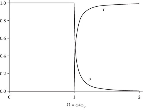
FIGURE 9.5
Sketch of the power reflection coefficient (ρ) and the power transmission coefficient (τ) of a plasma half-space.
Metals at optical frequencies are modeled as plasmas with plasma frequency ωp of the order of 1016. Refining the plasma model by including the collision frequency will lead to three frequency domains of conducting, cutoff, and dielectric phenomena [2]. A more comprehensive account of modeling metals as plasmas is given in References [3,4]. The associated phenomena of attenuated total reflection, surface plasmons, and other interesting topics are based on modeling metals as plasmas. A brief account of surface wave is given in Section 9.8.
9.4Reflection by a Plasma Slab [5]
In this section, we will consider oblique incidence to add to the variety to the problem formulation. The geometry of the problem is shown in Figure 9.6. Let x–z be the plane of incidence and ˆk be the unit vector along the direction of propagation. Let the magnetic field HI be along y and the electric field EI lie entirely in the plane of incidence. Such a wave is described in the literature by various names: (1) p wave, (2) TM wave, and (3) parallel-polarized wave. Since the boundaries are at z = 0 and d, it is necessary to use x–y–z-coordinates in formulating the problem and express ˆk in terms of x- and z-coordinates. The problem, though one-dimensional, appears to be two-dimensional. Equation 9.51, Equation 9.52, Equation 9.53, Equation 9.54, Equation 9.55 and Equation 9.56 describe the incident wave:
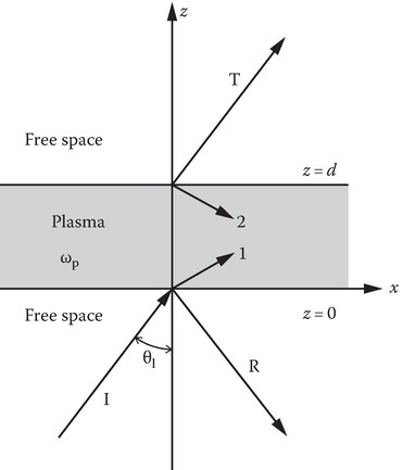
FIGURE 9.6
Plasma slab problem.
The reflected wave is written as
The boundary conditions at z = 0 require that the x dependence in the region z > 0 remains the same as in the region z < 0. Since the region z > d is also a free space, the exponential factor for the transmitted wave will be the same as the incident wave and the fields of the transmitted wave are
All the field amplitudes in the free space can be expressed in terms of EIx, ERx, or ETx:
We consider next the waves in the homogeneous plasma region 0 < z < d. The x and the z dependence for waves in the plasma comes from the exponential factor ΨP:
where q has to be determined. The wave number in the plasma is given as kp=k0√εp. Thus, we have
The two values for q indicate the excitation of two waves in the plasma, the first is the positive wave and the second is a negative wave. For Ω < 1/C, q is imaginary and the two waves in the plasma are evanescent. The next section deals with this frequency band.
The fields in the plasma can be written as
All the field amplitudes in the plasma can be expressed in terms of EPx1 and EPx2:
The above relations are obtained from Equations 9.3 and 9.6 by noting ∂/∂x = − jk0S and ∂/∂z = − jk0q; they can also be written from inspection. Assuming that EIx is known, the unknowns reduce to four, that is, EPx1, EPx2, ERx, and ETx. They can be determined from the four boundary conditions of continuity of the tangential components Ex and Hy at z = 0 and z = d. In matrix form,
where
Solving Equation 9.75,
where
The power reflection coefficient ρ=|ERx/EIx|2 is given by
where
In the above, λp is the free space wavelength corresponding to the plasma frequency and is used to normalize the slab width. Substituting for q1, in the range of real q1,
and in the range of imaginary q1,
where A and B are given by
The power transmission coefficient τ = (1 − ρ) and is given by
From Equation 9.85, ρ = 0 when sin A = 0 or
There is one more value of Ω for which ρ = 0. From Equation 9.88, when Cεp = q1, B = ∞, and from Equation 9.89, τ = 1 and ρ = 0. This point corresponds to a frequency ΩB given by
It is easily shown that ΩB exists only for the p wave and is greater than 1/C. In fact, this point corresponds to the Brewster angle [4]. Figure 9.7 shows ΩB versus cos θB, where θB is the Brewster angle.
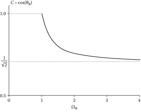
FIGURE 9.7
Brewster angle for a plasma medium.
Thus, in the frequency band Ω > 1/C, the variation of ρ with the slab width is oscillatory. Stratton [6] discussed these oscillations for a dielectric slab and associated them with the interference of the internally reflected waves in the slab. In the case of the plasma slab, the variation of ρ with the source frequency is also oscillatory, since in this range the plasma behaves like a dispersive dielectric. The maxima of ρ are less than or equal to 1 and occur for Ω satisfying the transcendental equation
where
Figure 9.8 shows ρ versus Ω for a normalized slab width dp = 1.0 and C = 0.5 (θI = 60°). The inset shows the variation of q with Ω. The oscillations can be clearly seen in the real range of q. Heald and Wharton [2] show similar curves for normal incidence on a lossy plasma slab using parameters normalized with reference to the source wave quantities.
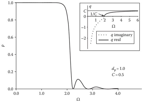
FIGURE 9.8
ρ versus Ω for isotropic plasma slab (parallel polarization).
In Figure 9.8, ρ ≈ 1 in the imaginary range of q showing total reflection of the source wave. However, it will be shown that there can be a considerable tunneling of power for sufficiently thin plasma slabs.
9.5Tunneling of Power through a Plasma Slab [5, 7]
For the frequency band Ω < 1/C, the characteristic roots are imaginary and the waves excited in the plasma are evanescent. The incident wave is completely reflected by the semi-infinite plasma. However, in the case of a plasma slab, some power gets transmitted through it even in this frequency band. It can be shown that this tunneling effect is due to the interaction of the electric field of the positive wave with the magnetic field of the negative wave and vice versa.
The above statement is supported by examining the power flow through the Poynting vector calculation. From Equation 9.77, Equation 9.78, Equation 9.79, Equation 9.80 and Equation 9.81, one can obtain
where
The magnetic field components HPy1, HPy2, and HTy can be obtained from Equations 9.65 and 9.73.
The power crossing any plane in the plasma parallel to the interface can be found by calculating the z-component of the Poynting vector associated with the plasma waves. This is given by
which on expansion gives
where ΨP1 and ΨP2 are given by Equation 9.72. The contribution from each of the four terms on the RHS of Equation 9.100 is now discussed for the two cases of q1 real Ω > 1/C and q1 imaginary Ω < 1/C. It is to be noted that the second and the third terms give the contributions due to the cross-interaction of the fields in the positive and negative waves.
Case 1: q1 real
It is easy to see that the second and the third terms being equal but opposite in sign, there is no contribution to the net power flow from the cross-interaction. The sum of the first and fourth terms is equal to (1/2)Re[(ETxΨT)(HT*yΨT*)], where ΨT is given by Equation 9.62. Thus, the power crossing any plane parallel to the slab interface gives exactly the power that emerges into the free space at the other boundary of the slab.
Case 2: q1 imaginary
It can be shown that each of the first and the fourth terms is zero. This is because the corresponding electric and magnetic fields are in time quadrature. Furthermore, the second term is equal to the third term and each is equal to (1/4)Re[(ETxΨT)(HT*yΨT*)]. Thus, the power flow in the tunneling frequency band (Ω < 1/C) comes entirely from the cross-interaction.
At Ω = 1, εp = 0, and from Equation 9.88, B = 0 but A ≠ 0. From Equation 9.89, τ = 0. This point exists only for the p wave.
At Ω = 1/C, A = 0, and B = 0. Evaluating the limit, we get the power transmission coefficient τc at this point:
Numerical results of τ versus Ω are presented in Figures 9.9 and 9.10 for the tunneling frequency band. In Figure 9.9, the angle of incidence is taken to be 60° and the curves are given for various dp. Between Ω = 0 and 1, there is a value of Ω = Ωmax where the transmission is maximum. The maximum value of the transmitted power decreases as dp increases.
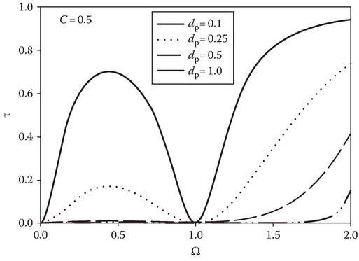
FIGURE 9.9
Transmitted power for an isotropic plasma slab (parallel polarization) in the tunneling range (Ω < 1/C) for various dp. The right side of the bottom two curves can be seen more clearly than the left side and they are for dp = 0.5 and dp = 1.0.
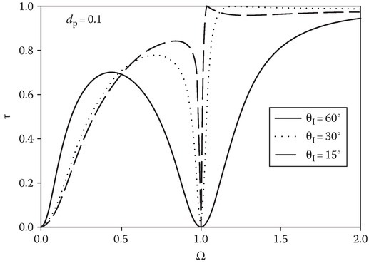
FIGURE 9.10
Transmitted power for an isotropic plasma slab (parallel polarization) in the tunneling range (Ω < 1/C) for various angles of incidence. The broken line curve is for θI = 15°.
In Figure 9.10, τ versus Ω is shown with the angle of incidence as the parameter. It is seen that the point of maximum transmission moves to the right as the angle of incidence decreases and merges with Ω = 1 for θI = 0° (normal incidence). The maximum value of the transmitted power decreases as θI increases. This point is given by the solution of the transcendental equation
where f and A are given in Equations 9.94 and 9.87, respectively. It is suggested that by measuring Ωmax experimentally, one can determine either the plasma frequency or the slab width, knowing the angle of incidence.
9.6Inhomogeneous Slab Problem
Let us next consider the case where εp is a function of z in the region 0 < z < d. To simplify and focus on the effect of the inhomogeneity of the properties of the medium, let us revert to the normal incidence. The differential equation for the electric field is given by Equation 9.15. This equation cannot be solved exactly for a general εp(z) profile.
However, there are a small number of profiles for which exact solutions can be obtained in terms of special functions. As an example, the problem of the linear profile can be solved in terms of Airy functions. An account of such solutions for a dielectric profile εr(z) are given in [8,9] and for a plasma profile εp(z, ω) in [2,10]. Abramowitz and Stegun [11] give detailed information on special functions.
A vast amount of literature is available on the approximate solution for an inhomogeneous media problem. The following techniques are emphasized in this book. The actual profile is considered as a perturbation of a profile for which the exact solution is known. The effect of the perturbation is calculated through the use of Green’s function. The problem of a fast profile with finite range—length can be so handled by using a step profile as the reference. At the other end of the approximation scale, the slow profile problem can be handled by adiabatic and WKBJ techniques. See [1,8] for dielectric profile examples and [2,10] for plasma profile examples. Numerical approximation techniques can also be used which are extremely useful in obtaining specific numbers for a given problem and in validating the theoretical results obtained from the physical approximations.
9.7Periodic Layers of Plasma
Next, we consider a particular case of an inhomogeneous plasma medium which is periodic. Let the dielectric function
where m is an integer and L is the spatial period. If the domain of m is all integers, −∞ < m < ∞, then we have an unbounded periodic media. The solution of Equation 9.15 for the infinite periodic structure problem [1,9,12] will be such that the electric field E(z) differs from the electric field at E(z + L) by a constant:
The complex constant C be written as
where β is the complex propagation constant of the periodic media. Thus, one can write
From Equation 9.106,
Also from Equations 9.104 and 9.106,
From Equations 9.107 and 9.108, it follows that Eβ(z) is periodic:
Equation 9.106, where Eβ(z) is periodic, is called the Bloch wave condition. Such a periodic function can be expanded in a Fourier series:
and E(z) can be written as
where
Taking into account both positive-going and negative-going waves, E(z) can be expressed as [1]
Let us next consider the wave propagation in a periodic layered media with plasma layers alternating with the free space. The geometry of the problem is shown in Figure 9.11. Adopting the notation of [12] a unit cell consists of free space from −l < z < l and a plasma layer of plasma frequency ωp0 from l < z < l + d. The thickness of the unit cell is L = 2l + d. The electric field E(z) in the two layers of the unit cell can be written as
where n is the refractive index of the plasma medium:
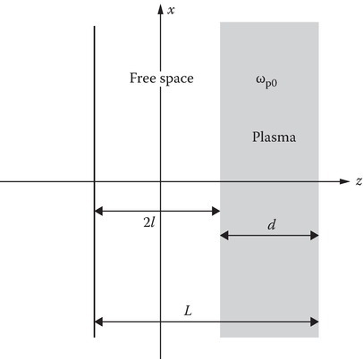
FIGURE 9.11
Unit cell of unbounded periodic media consisting of layer of plasma.
The continuity of tangential electric and magnetic fields at the boundary translates into the continuity of E and ∂E/∂z at the interfaces:
From Equations 9.117 and 9.118,
Since l + d+ = −l+ + L, from Equation 9.104,
From Equations 9.114, 9.115, 9.119, and 9.123
From Equations 9.114, 9.115, 9.120, and 9.123
Equations 9.121, 9.122, 9.124, and 9.125 can be arranged as a matrix as
A nonzero solution for the fields can be obtained by equating the determinant of the square matrix in Equation 9.126 to zero. This leads to the dispersion relation
Section 7.4 gives an alternative way of obtaining the dispersion relation based on transmission line analogy and the ABCD parameters.
The above equation can be studied by using reference values βr and ωr = βrc = 2πc/λr. Thus, Equation 9.127, in the normalized form, can be written as
Figure 9.12 shows the graph ω/ωr versus β/βr for the following values of the parameters: L = 0.6λr, d = 0.2λr, and ωp0 = 1.2ωr. We note from Figure 9.12 that the wave is evanescent in the frequency band 0 < ω/ωr < 0.611. This stop band is due to the plasma medium in the layers. If the layers are dielectric, this stop band will not be present. We have again a stop band in the frequency domain 0.877 < ω/ωr < 1.225. This stop band is due to the periodicity of the medium. Periodic dielectric layers do exhibit such a forbidden band. This principle is used in optics to construct Bragg reflectors with extremely large reflectance [9]. Figure 9.13 shows the ω–β diagram for dielectric layers with the refractive index n = 1.8. The first stop band in this case is given by 0.537 < ω/ωr < 0.779.
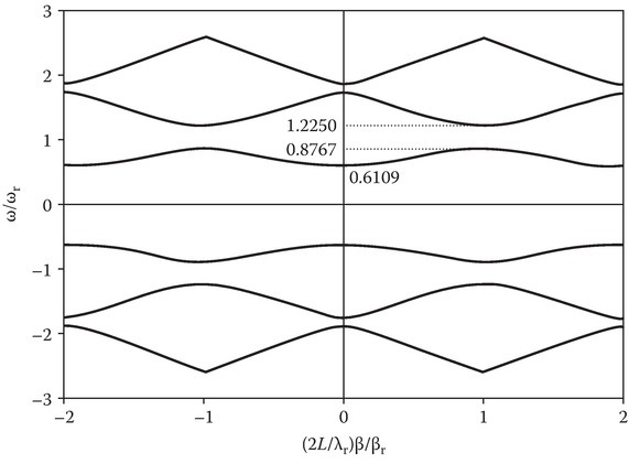
FIGURE 9.12
Dispersion relation of a periodic plasma medium for d = 0.2λr and L = 0.6λr.

FIGURE 9.13
Dispersion relation of periodic dielectric layers for d = 0.2λr and L = 0.6λr. The refractive index of the dielectric layer is 1.8.
9.8Surface Waves
Let us backtrack a little bit and consider the oblique incidence of a p wave on a plasma half-space. In this case, only the outgoing wave will be excited in the plasma half-space and Equation 9.75 becomes
Solution of Equation 9.129 gives the fields of the reflected wave and the wave in the plasma half-space in terms of the fields of the incident wave. If is zero (no incident wave), we expect . This is true in general with one exception. The exception occurs when the determinant of the square matrix on the LHS of Equation 9.129 is zero. In such a case, and can be nonzero even if is zero, indicating the possibility of the existence of fields in free space even if there is no incident field. For the exceptional solution, the reflection coefficient is infinity, that is, , but . The solution is an eigenvalue solution and gives the dispersion relation for surface plasmons. From Equations 9.73 and 9.129, the dispersion relation is obtained as
Noting that
and
where
the dispersion relation can be written as
The exponential factors for z < 0 and z > 0 can be written as
It can be shown that kx will be real and both
and
will be real and positive if
When Equation 9.140 is satisfied
where α1 and α2 are positive real quantities. Equations 9.141 and 9.142 show that the waves, while propagating along the surface, attenuate in the direction normal to the surface. For this reason, the wave is called a surface wave. In a plasma when εp will be less than −1. Thus, an interface between free space and a plasma medium can support a surface wave.
Defining the refractive index of the surface mode as n, that is,
Equation 9.135 can be written as
For n is real and the surface wave propagates. In this interval of ω, the dielectric constant εp < −1. The surface wave mode is referred to, in the literature, as Fano mode [13] and also as a nonradiative surface plasmon. In the interval 1 < Ω < ∞, n2 is positive and less than 0.5. However, the α-values obtained from Equations 9.138 and 9.139 are imaginary. The wave is not bound to the interface and the mode, called Brewster mode, in this case is radiative and referred to as a radiative surface plasmon. Figure 9.14 sketches εp(ω) and n2 (ω). Another way of presenting the information is through the Ω−K diagram, where Ω and K are normalized frequency and wave number, respectively, that is,

FIGURE 9.14
Refractive index for surface plasmon modes.
From Equations 9.143 and 9.144, we obtain the relation
Figure 9.15 shows the Ω–K diagram.
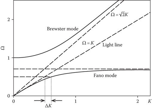
FIGURE 9.15
Ω−K diagram for surface plasmon modes.
The Fano mode is a surface wave called the surface plasmon and exists for The surface mode does not have a low-frequency cutoff. It is guided by an open-boundary structure. It has a phase velocity less than that of light. The eigenvalue spectrum is continuous. This is in contrast to the eigenvalue spectrum of a conducting-boundary waveguide that has an infinite number of discrete modes of propagation at a given frequency.
The application of photons (electromagnetic light waves) to excite the surface plasmons meets with the difficulty that the dispersion relation of the Fano mode lies to the right of the light line Ω = K (see Figure 9.15). At a given photon energy ℏω, the photon momentum ℏkx has to be increased by ℏΔkx = ℏ(ωp/c)ΔK in order to transform the photons into surface plasmons. The two techniques commonly used to excite surface plasmons are (a) grating coupler (b) attenuated total reflection (ATR) method. A complete account of surface plasmons can be found in [13,14].
Surface waves can also exist at the interface of a dielectric with a plasma layer or a plasma cylinder. The theory of surface waves on a gas-discharge plasma is given in [15]. Kalluri [16] used this theory to explore the possibility of a backscatter from a plasma plume see Appendix 9A for details. Moissan et al. [17] achieved plasma generation through surface plasmons in a device called Surfatron. It is a highly efficient device for launching surface plasmons that produce plasma at a microwave frequency.
9.9Transient Response of a Plasma Half-Space
Reflection of transient pulses from a sharply bounded plasma half-space can be obtained by finding the response of the plasma to a time-harmonic wave. For example, if R(jω) is the reflection coefficient, then the response to an impulsive plane wave er (t) can be obtained [18].
Let e0(t) = δ(t) be the electric field of the impulsive plane wave at z = 0. Its Laplace transform is
If the reflected field is designated at the point of incidence on the interface er (t), then its Laplace transform Er(s) is given by
where R(s) is obtained by replacing ( jω) by s in R(jω): the Laplace inverse of R(s) gives er(t):
A direct analytical evaluation of Equation 9.150 is modified to suit the numerical evaluation [19]
where is assumed er(t) = 0 for t < 0 and Re stands for real.
9.9.1Isotropic Plasma Half-Space s Wave
Consider oblique incidence of an s wave. It can be shown [18] that
where
and θ is the angle of incidence. From a standard Laplace transform table [11],
Thus, one obtains the Laplace inverse of Equation 9.153, leading to
Figure 9.16 shows the impulse response for various angles of incidence. The effect of dispersion is clearly visible. There is an appreciable effect of the angle of incidence on the amplitude and the period of oscillation of the response. It is seen that as the angle of incidence decreases (or C increases), the amplitude of the response (especially the early part) decreases, whereas the period of the oscillation increases. The variation of Re[R(Ω)] with Ω = ω/ωp is shown as an inset for C = 0.4.
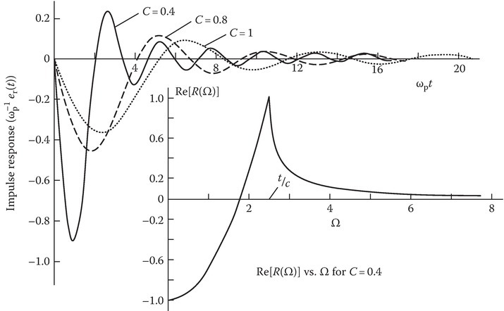
FIGURE 9.16
Impulse response of isotropic plasma half-space to an s-wave incidence.
9.9.2Impulse Response of Several Other Cases Including Plasma Slab
References [18,19,20,21,22,23,24,25,26] and the references in these citations give access to the additional literature on this topic.
9.10Solitons [27]
This topic deals with a desirable aspect of the EMW transformation by the balancing act of two complexities each of which by itself produces an undesirable effect. The balancing of the wave-breaking feature of a nonlinear medium complexity with the flattening feature of the dispersion leads to a soliton solution. Hirose and Longren [27] give a transmission line analogy to explain the balancing of the two dominant effects of the complexities of dispersion and nonlinearity. Ricketts and Ham [28] discuss the theory, design, and application of electrical solitons.
9.11Perfect Dispersive Medium
As we have seen in Figure 9.16, a dispersive medium distorts a pulse by modulating the instantaneous frequency contents of the pulse. Gupta and Caloz [29] have explained the concept of a perfect dispersive medium with a perfectly flat transmission coefficient magnitude over the entire spectrum leading to an improved real-time signal processing technology. It is an engineered medium of “stacked loss-gain metasurfaces” [29].
Several such new ideas are being pursued under the broad banner of dispersion-engineered space-time modulated systems.
References
- 1.Ishimaru, A., Electromagnetic Wave Propagation, Radiation, and Scattering, Prentice Hall, Englewood Cliffs, NJ, 1991.
- 2.Heald, M.A. and Wharton, C.B., Plasma Diagnostics with Microwaves, Wiley, New York, 1965.
- 3.Forstmann, F. and Gerhardts, R.R., Metal Optics Near the Plasma Frequency, Springer, New York, 1986.
- 4.Boardman, A.D., Electromagnetic Surface Modes, Wiley, New York, 1982.
- 5.Kalluri, D. K. and Prasad, R. C., Thin film reflection properties of isotropic and uniaxial plasma slabs, Appl. Sci. Res. (Netherlands), 27, 415, 1973.
- 6.Stratton, J.A., Electromagnetic Theory, McGraw-Hill, New York, 1941.
- 7.Kalluri, D. K. and Prasad, R. C., Transmission of power by evanescent waves through a plasma slab, 1980 IEEE International Conference on Plasma Science, Madison, WI, p. 11, May 19–21, 1980.
- 8.Lekner, J., Theory of Reflection, Kluwer, Boston, MA, 1987.
- 9.Yeh, P., Optical Waves in Layered Media, Wiley, New York, 1988.
- 10.Budden, K.G., Radio Waves in the Ionosphere, Cambridge University Press, Cambridge, U.K., 1961.
- 11.Abramowitz, M. and Stegun, I.A., Handbook of Mathematical Functions, Dover Publications, New York, 1965.
- 12.Kuo, S.P. and Faith, J., Interaction of an electromagnetic wave with a rapidly created spatially periodic plasma, Phys.Rev.E, 56, 1, 1997.
- 13.Boardman, A.D., Hydrodynamic theory of plasmon–polaritons on plane surfaces, in: Boardman, A. D. (Ed.), Electromagnetic Surface Modes, Wiley, New York, 1982, Chap. 1, pp. 1–76.
- 14.Raether, H., Surface Plasmons, Springer, New York, 1988.
- 15.Shivarova, A. and Zhelyazkov, I., Surface waves in gas-discharge plasmas, in: Boardman, A.D. (Ed.), Electromagnetic Surface Modes, Wiley, New York, 1982, Chap.12.
- 16.Kalluri, D.K., Backscattering from a plasma plume due to excitation of surface waves, Final Report Summer Faculty Research Program, Air Force Office of Scientific Research, Arlington Virginia, 1994.
- 17.Moissan, C., Beandry, C., and Leprince, P., Phys.Lett., 50A, 125, 1974.
- 18.Prasad, R.C., Transient and frequency response of a bounded plasma, Doctoral thesis, Birla Institute of Technology, Ranchi, India, 1976.
- 19.Ley, B.J., Computer Aided Analysis and Design for Electrical Engineering, Holt, Rinehart and Winston, New York, 1970.
- 20.Kalluri, D. and Prasad, R.C., Transient response of a cold lossless plasma half-space in the presence of transverse static magnetic field, J. Appl. Phys., 49(6), 3593–3594, 1978.
- 21.Kalluri, D. and Prasad, R.C., Reflection of an impulsive plane wave by a plasma half-space moving perpendicular to the plane of incidence, J. Appl. Phys., 49(5), 2696–2699, 1978.
- 22.Prasad, R.C. and Kalluri, D., Reflection of an obliquely incident impulsive plane wave from isotropic and uniaxial cold lossy plasma half-spaces, IEEE Trans. Plasma Sci., PS-6(4), 543–549, 1978.
- 23.Kalluri, D. and Prasad, R.C., On impulse response of plasma half-space moving normal to the interface-I: Formulation of the solution, 1979 IEEE International Conference on Plasma Science, Montreal, Quebec, Canada, Conference Record-Abstracts, June 4–6, 1979, p. 155.
- 24.Kalluri, D. and Prasad, R.C., On impulse response of plasma half-space moving normal to the interface-II: Results, 1979 IEEE International Conference on Plasma Science, Montreal, Quebec, Canada, Conference Record-Abstracts, June 4–6, 1979, pp. 154–155.
- 25.Kalluri, D. and Prasad, R.C., Transient response of a cold lossless plasma half-space in the presence of transverse static magnetic field, J. Appl. Phys., 50(4), 2959–2961, 1979.
- 26.Prasad, R.C. and Kalluri, D., Impulse response of a lossy magnetoplasma half-space moving along the magnetic field, 1980 IEEE International Conference on Plasma Science, Madison, WI, Conference Record-Abstracts, May 19–21, 1980, pp. 11–12.
- 27.Hirose, A. and Longren, K.E., Introduction to Wave Phenomena, Wiley, New York, 1985.
- 28.Ricketts, D.S. and Ham, D., Electrical Solitons, CRC Press, Boca Raton, FL, 2011.
- 29.Gupta, S., and Caloz, C., Perfect dispersive medium for real-time signal processing, IEEE Trans.Antennas Propag., 64(12), 5299–5308, December 2016.