In the following section, we will learn the implementation of the previously described models with the help of R.
In Chapter 4, Big Data – Advanced Analytics, we will discuss in detail the aspects and methods of getting data from open sources and working with them efficiently. Here, we only present how the time series of stock prices and other relevant information can be acquired and used for the factor model's estimations.
We used the quantmod package to collect the database.
Here is how it works in R:
library(quantmod)
stocks <- stockSymbols()
As a result, we need to wait for a few seconds while data is fetched, and then we can see the output:
Fetching AMEX symbols...
Fetching NASDAQ symbols...
Fetching NYSE symbols...
Now, we have a data frame R object that contains about 6,500 stocks that are traded on different exchanges such as AMEX, NASDAQ, or NYSE. In order to see the variables that the dataset contains, we can use the str command:
str(stocks)
'data.frame':   6551 obs. of  8 variables:
 $ Symbol   : chr  "AA-P" "AAMC" "AAU" "ACU" ...
 $ Name     : chr  "Alcoa Inc." "Altisource Asset Management Corp"...
 $ LastSale : num  87 1089.9 1.45 16.58 16.26 ...
 $ MarketCap: num  0.00 2.44e+09 9.35e+07 5.33e+07 2.51e+07 ...
 $ IPOyear  : int  NA NA NA 1988 NA NA NA NA NA NA ...
 $ Sector   : chr  "Capital Goods" "Finance" "Basic Industries"...
 $ Industry : chr  "Metal Fabrications" "Real Estate"...
 $ Exchange : chr  "AMEX" "AMEX" "AMEX" "AMEX" ...
We can drop the variables that we don't really need and include the information about market capitalization and the book value of the company coming from a different database as new variables since we will need them to estimate the Fama-French model:
stocks[1:5, c(1, 3:4, ncol(stocks))]
      Symbol LastSale  MarketCap BookValuePerShare
1   AA-P    87.30          0              0.03
2   AAMC   985.00 2207480545            -11.41
3    AAU     1.29   83209284              0.68
4    ACU    16.50   53003808             10.95
5    ACY    16.40   25309415             30.13
We will also need the time series of the risk-free return, which will be quantified in this calculation by the one-month USD LIBOR rate:
library(Quandl)
Warning message:
package 'Quandl' was built under R version 3.1.0
LIBOR <- Quandl('FED/RILSPDEPM01_N_B',
start_date = '2010-06-01', end_date = '2014-06-01')
Warning message:
In Quandl("FED/RILSPDEPM01_N_B", start_date = "2010-06-01", end_date = "2014-06-01") : It would appear you aren't using an authentication token. Please visit http://www.quandl.com/help/r or your usage may be limited.
We can ignore the warning messages as data is still assigned to the LIBOR variable.
The Quandl package, the tseries package, and other packages that collect data are discussed in Chapter 4, Big Data – Advanced Analytics, in more detail.
This can also be used to get the prices of stocks, and the S&P 500 index can be used as the market portfolio.
We have a table with stock prices (a time series of approximately 5,000 stock prices between June 1, 2010 to June 1, 2014). The first and last few columns look like this:
d <- read.table("data.csv", header = TRUE, sep = ";")
d[1:7, c(1:5, (ncol(d) - 6):ncol(d))]
         Date       SP500  AAU   ACU   ACY   ZMH   ZNH ZOES  ZQK ZTS ZX
1  2010.06.01 1070.71 0.96 11.30 20.64 54.17 21.55  NA  4.45 NA NA
2  2010.06.02 1098.38 0.95 11.70 20.85 55.10 21.79  NA  4.65 NA NA
3  2010.06.03 1102.83 0.97 11.86 20.90 55.23 21.63  NA  4.63 NA NA
4  2010.06.04 1064.88 0.93 11.65 18.95 53.18 20.88  NA  4.73 NA NA
5  2010.06.07 1050.47 0.97 11.45 19.03 52.66 20.24  NA  4.18 NA NA
6  2010.06.08 1062.00 0.98 11.35 18.25 52.99 20.96  NA  3.96 NA NA
7  2010.06.09 1055.69 0.98 11.90 18.35 53.22 20.45  NA  4.02 NA NA
If we have the data saved on our hard drive, we can simply read it with the read.table function. In Chapter 4, Big Data – Advanced Analytics, we will discuss how to collect data directly from the Internet.
Now, we have all the data we need: the market portfolio (S&P 500), the price of stocks, and the risk-free rates (one-month LIBOR).
We have chosen to delete the variables with missing values and 0 or negative prices, in order to clean the database. The easiest way to do this is the following:
d <- d[, colSums(is.na(d)) == 0]
d <- d[, c(T, colMins(d[, 2:ncol(d)]) > 0)]
To use the colMins function, we apply the matrixStats package. Now, we can start working with the data.
In practice, it is not easy to carry out a factor analysis, because identifying the macro variables that have an effect on the securities' return is difficult (Medvegyev – Száz, 2010, pp. 42). In many cases, the latent factors that drive the returns are searched by principal component analysis.
From the originally downloaded 6,500 stocks, we can use the data of 4,015 stocks; the rest were excluded because of missing values or 0 prices. Now, we omit the first two columns because we do not need the dates in this section, and the S&P 500 is considered as a separate factor in itself; hence, we do not include it in the principal component analysis (PCA). After this, the log returns are computed.
p <- d[, 3:ncol(d)]
r <- log(p[2:nrow(p), ] / p[1:(nrow(p) - 1), ])
There exists another way to calculate the log returns of a given asset, that is, by using return.calculate(data, method="log") with the PerformanceAnalytics library.
As we have too many stocks, in order to carry out PCA, either we have to have data of at least 25 years, or we need to reduce the number of stocks. It's hopeless for factor models to remain stable for decades; hence, for illustration purposes, we choose to select 10 percent of the stocks randomly and compute the model for this sample:
r <- r[, runif(nrow(r)) < 0.1]
runif(nrow(r)) < 0.1 is a 4,013 dimension 0-1 vector, which chooses approximately 10 percent of the columns (in our case, 393) from the table. We can also use the following sample function for this, on which you can find further details at http://stat.ethz.ch/R-manual/R-devel/library/base/html/sample.html:
pca <- princomp(r)
As a result, we receive a princomp class object, which has eight attributes, of which the most important ones are the loading matrix and the sdev attributes, which contain the standard deviations of the components. The first principal component is the vector on which the data set has the maximum variance.
Let's check the standard deviations of the principal component:
plot(pca$sdev)
The result is as follows:
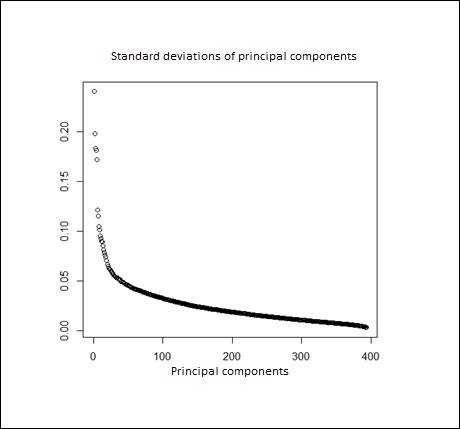
We can see that the first five components are separated; consequently, five factors should be chosen, but other factors also have significant standard deviations, so the market cannot be explained by a few factors.
We can confirm this result by calling the factanal function, which estimates the factor model with five factors:
factanal(r, 5)
We notice that it takes much more time to perform this computation. Factor analysis is related to PCA, but is a little more complicated from a mathematical aspect. As a result, we get an object of class factanal, which has many attributes, but now, we are only interested in the following part of the output:
               Factor1 Factor2 Factor3 Factor4 Factor5
SS loadings     56.474  23.631  15.440  12.092   6.257
Proportion Var   0.144   0.060   0.039   0.031   0.016
Cumulative Var   0.144   0.204   0.243   0.274   0.290
Test of the hypothesis that 5 factors are sufficient.
The chi square statistic is 91756.72 on 75073 degrees of freedom.The p-value is 0
This output shows that the factor model with five factors fits, but the explained variance is only approximately 30 percent, which means that the model should be extended with other factors as well.
We have a data frame with prices of the 4,015 stocks for five years, and the LIBOR data frame with the LIBOR time series. First, we need to compute the returns and combine them with the LIBOR rate.
As a first step, we omit the dates that are not for mathematical computations, and then we compute the log returns for each of the remaining columns:
d2 <- d[, 2:ncol(d)]
d2 <- log(tail(d1, -1)/head(d1, -1))
After calculating the log returns, we put back the dates to the returns, and then, as a last step, we combine the two data sets:
d <- cbind(d[2:nrow(d), 1], d2)
d <- merge(LIBOR, d, by = 1)
It is worth mentioning that the merge function operates on data frames equivalent to the (inner) join SQL statement.
The result is as follows:
print(d[1:5, 1:5])]
     Date   LIBOR      SP500                AAU             ACU
2010.06.02   0.4        0.025514387    -0.01047130     0.034786116
2010.06.03   0.4        0.004043236     0.02083409      0.013582552
2010.06.04   0.4       -0.035017487    -0.04211149    -0.017865214
2010.06.07   0.4       -0.013624434     0.04211149    -0.017316450
2010.06.08   0.4        0.010916240     0.01025650     -0.008771986
We adjust the LIBOR rate to the daily returns:
d$LIBOR <- d$LIBOR / 36000
As the LIBOR rates are quoted on a money-market basis - (actual/360) day-count convention - and the time series contain the rates in percentage, we divided the LIBOR by 36,000. Now, we need to compute the three variables of the Fama-French model. As described in the Data selection section, we have the stocks' data frame:
d[1:5, c(1,(ncol(d) - 3):ncol(d))]
  Symbol LastSale  MarketCap BookValuePerShare
1   AA-P    87.30          0              0.03
2   AAMC   985.00 2207480545            -11.41
3    AAU     1.29   83209284              0.68
4    ACU    16.50   53003808             10.95
5    ACY    16.40   25309415             30.13
We have to drop the stocks for which we do not have price data:
> stocks = stocks[stocks$Symbol %in% colnames(d),]
We have the market cap as a variable; we still need to compute the book-to-market ratio for each:
stocks$BookToMarketRatio <-
  stocks$BookValuePerShare / stocks$LastSale
str(stocks)
'data.frame':   3982 obs. of  5 variables:
 $ Symbol           : Factor w/ 6551 levels "A","AA","AA-P",..: 14 72...
 $ LastSale         : num  1.29 16.5 16.4 2.32 4.05 ...
 $ MarketCap        : num  8.32e+07 5.30e+07 2.53e+07 1.16e+08...
 $ BookValuePerShare: num  0.68 10.95 30.13 0.19 0.7 ...
 $ BookToMarketRatio: num  0.5271 0.6636 1.8372 0.0819 0.1728 ...
Now, we need to compute the SMB and HML factors. For simplification, we will define companies as BIG if they are bigger than the average. The same principle is applied for the book-to-market ratio:
avg_size <- mean(stocks$MarketCap)
BIG   <- as.character(stocks$Symbol[stocks$MarketCap > avg_size])
SMALL <- as.character(stocks[stocks$MarketCap < avg_size,1])
These arrays contain the symbols of the BIG and SMALL companies. Now, we can define the SMB factor:
d$SMB <- rowMeans(d[,colnames(d) %in% SMALL]) –
  rowMeans(d[,colnames(d) %in% BIG])
We define the HML factor as follows:
avg_btm <- mean(stocks$BookToMarketRatio)
HIGH <- as.character(
  stocks[stocks$BookToMarketRatio > avg_btm, 1])
LOW <- as.character(
  stocks[stocks$BookToMarketRatio < avg_btm, 1])
d$HML <- rowMeans(d[, colnames(d) %in% HIGH]) –
  rowMeans(d[, colnames(d) %in% LOW])
The third factor is calculated:
d$Market <- d$SP500 - d$LIBOR
After defining the three factors, we test it on the stock of Citigroup Inc. (Citi) and on Exelixis, Inc. (EXEL):
d$C   <- d$C - d$LIBOR
model <- glm( formula = "C ~ Market + SMB + HML" , data = d)
The GLM (general linear model) function works as follows: it takes the data and formula as arguments. The formula is a string in the form of response ~ terms, where the response is a variable name in the data frame and terms specify the predictors in the model, so it consists of variable names in the data set separated by + operators. This function can also be used for logistic regression, but the default is linear.
The output of the model is as follows:
Call:  glm(formula = "C~Market+SMB+HML", data = d)
Coefficients:
(Intercept)       Market          SMB          HML
   0.001476     1.879100     0.401547    -0.263599
Degrees of Freedom: 1001 Total (i.e. Null);  998 Residual
Null Deviance:      5.74
Residual Deviance: 5.364        AIC: -2387
The output of the model summary is as follows:
summary(model)
Call:
glm(formula = "C~Market+SMB+HML", data = d)
Deviance Residuals:
     Min        1Q    Median        3Q       Max
-0.09344  -0.01104  -0.00289   0.00604   2.26882
Coefficients:
             Estimate Std. Error t value Pr(>|t|)
(Intercept)  0.001476   0.002321   0.636    0.525
Market       1.879100   0.231595   8.114 1.43e-15 ***
SMB          0.401547   0.670443   0.599    0.549
HML         -0.263599   0.480205  -0.549    0.583
---
Signif. codes:  0 '***' 0.001 '**' 0.01 '*' 0.05 '.' 0.1 ' ' 1
(Dispersion parameter for gaussian family taken to be 0.005374535)
    Null deviance: 5.7397  on 1001  degrees of freedom
Residual deviance: 5.3638  on  998  degrees of freedom
AIC: -2387
Number of Fisher Scoring iterations: 2
The results show that the only significant factor is the market premium, which means that the stock return of Citigroup seems to moves together with the whole market itself.
To plot the results, this command should be used:
estimation <- model$coefficients[1]+
  model$coefficients[2] * d$Market +
  model$coefficients[3]*d$SMB +
  model$coefficients[4]*d$HML
plot(estimation, d$C, xlab = "estimated risk-premium",
  ylab = "observed riks premium",
  main = "Fama-French model for Citigroup")
lines(c(-1, 1), c(-1, 1), col = "red")
The following screenshot shows an estimated risk premium of the Fama-French model for Citigroup:
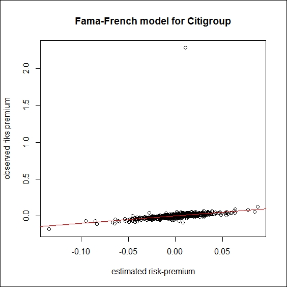
If we have a look at the graph we can see that we have an outlier in the returns. Let’s see what happens if we get rid of it, by replacing it with 0.
outlier <- which.max(d$C)
d$C[outlier] <- 0
If we run the same code again to create the model, and calculate the estimated and observed returns again we get the following results:
model_new <- glm( formula = "C ~ Market + SMB + HML" , data = d)
summary(model_new)
Call:
glm(formula = "C ~ Market + SMB + HML", data = d)
Deviance Residuals:
      Min         1Q     Median         3Q        Max
-0.091733  -0.007827  -0.000633   0.007972   0.075853
Coefficients:
              Estimate Std. Error t value Pr(>|t|)
(Intercept) -0.0000864  0.0004498  -0.192 0.847703
Market       2.0726607  0.0526659  39.355  < 2e-16 ***
SMB          0.4275055  0.1252917   3.412 0.000671 ***
HML          1.7601956  0.2031631   8.664  < 2e-16 ***
---
Signif. codes:  0 ‘***’ 0.001 ‘**’ 0.01 ‘*’ 0.05 ‘.’ 0.1 ‘ ’ 1
(Dispersion parameter for gaussian family taken to be 0.0001955113)
    Null deviance: 0.55073  on 1001  degrees of freedom
Residual deviance: 0.19512  on  998  degrees of freedom
AIC: -5707.4
Number of Fisher Scoring iterations: 2
According to the results, the all the three factors are significant.
The GLM function does not return R2. For linear regression, the lm function can be used exactly the same way, and we can get from model summary r.squared = 0.6446.
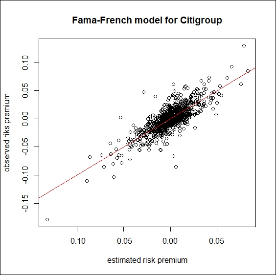
This result indicates that the variables explain more than 64 percent of the variance of the risk-premium of Citi. Let’s plot the new results:
estimation_new <- model_new$coefficients[1]+
  model_new$coefficients[2] * d$Market +
  model_new$coefficients[3]*d$SMB +
  model_new$coefficients[4]*d$HML
dev.new()
plot(estimation_new, d$C, xlab = "estimated risk-premium",ylab = "observed riks premium",main = "Fama-French model for Citigroup")
lines(c(-1, 1), c(-1, 1), col = "red")
The output in this case is the following:
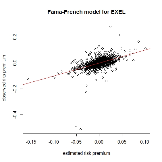
We test the model on another stock, EXEL, as well:
d$EXEL <- d$EXEL – d$LIBOR
model2 <- glm( formula = "EXEL~Market+SMB+HML" , data = d)
Call:  glm(formula = "EXEL~Market+SMB+HML", data = d)
Coefficients:
(Intercept)       Market          SMB          HML
  -0.001048     2.038001     2.807804    -0.354592
Degrees of Freedom: 1001 Total (i.e. Null);  998 Residual
Null Deviance:      1.868
Residual Deviance: 1.364        AIC: -3759
The output for the model summary is as follows:
summary(model2)
Call:
glm(formula = "EXEL~Market+SMB+HML", data = d)
Deviance Residuals:
     Min        1Q    Median        3Q       Max
-0.47367  -0.01480  -0.00088   0.01500   0.25348
Coefficients:
             Estimate Std. Error t value Pr(>|t|)
(Intercept) -0.001773   0.001185  -1.495  0.13515
Market       1.843306   0.138801  13.280  < 2e-16 ***
SMB          2.939550   0.330207   8.902  < 2e-16 ***
HML         -1.603046   0.535437  -2.994  0.00282 **
---
Signif. codes:  0 ‘***’ 0.001 ‘**’ 0.01 ‘*’ 0.05 ‘.’ 0.1 ‘ ’ 1

(Dispersion parameter for gaussian family taken to be 0.001357998)
    Null deviance: 1.8681  on 1001  degrees of freedom
Residual deviance: 1.3553  on  998  degrees of freedom
AIC: -3765.4
Number of Fisher Scoring iterations: 2
According to the results, all of the three factors are significant.
The GLM function does not contain R2. For linear regression, the lm function can be used exactly the same way, and we get r.squared = 0.2723 from model summary. Based on the results, the variables explain more than 27 percent of the variance of the risk premium of EXEL.
To plot the results, the following command can be used:
estimation2 <- model2$coefficients[1] +
  model2$coefficients[2] * d$Market +
  model2$coefficients[3] * d$SMB + model2$coefficients[4] * d$HML
plot(estimation2, d$EXEL, xlab = "estimated risk-premium",
  ylab = "observed riks premium",
  main = "Fama-French model for EXEL")
lines(c(-1, 1), c(-1, 1), col = "red")