
Financial risk is a tangible and quantifiable concept, a value that you can lose on a certain financial investment. Note that here, we strictly differentiate between uncertainty and risk, where the latter is measurable with mathematical-statistical methods with exact probabilities of the different outcomes. However, there are various kinds of measures for financial risks. The most common risk measure is the standard deviation of the returns of a certain financial instrument. Although it is very widespread and easy to use, it has some major disadvantages. One of the most important problems of the standard deviation as a risk measurement is that it treats upside potential the same way as downside risk. In other words, it also punishes a financial instrument that might bring huge positive returns and little negative ones than a less volatile asset.
Consider the following extreme example. Let's assume that we have two stocks on the stock market and we can exactly measure the stocks' yields in three different macroeconomic events. Next year for stock A, a share of a mature corporation brings 5 percent yield if the economy grows, 0 percent if there is stagnation, and loses 5 percent if there's a recession. Stock B is a share of a promising start-up firm; it skyrockets (+ 50 percent) when there's a good economic environment, brings 30 percent if there's stagnation, and has a 20 percent annual yield even if the economy contracts. The statistical standard deviations of stock A and B's returns are 4.1 percent and 12.5 percent respectively. Therefore, it is riskier to pick stock A than stock B if we make our choice based on the standard deviation. However, using our common sense, it is obvious that stock B is better in every case than stock A as it gives a better yield in all different macroeconomic situations.
Our short example perfectly showed the biggest problem with standard deviation as a risk measure. The standard deviation does not meet the most simple condition of a coherent risk measure, the monotonicity. We call the σ risk measure coherent if it is normalized and meets the following criteria. See the work of Artzner and Delbaen for further information on coherent risk measures:
- Monotonicity: If portfolio X1 has no lower values than portfolio X2 under all scenarios, then the risk of X1 should be lower than X2. In other words, if an instrument pays more than another one in every case, it should have a lower risk.

- Sub-additivity: The risk of two portfolios together should be less than the sum of the risks of the two portfolios separately. This criterion represents the principle of diversification.

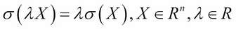
- Positive homogeneity: Multiplying the portfolio values by a constant multiplies the risk by the same extent.
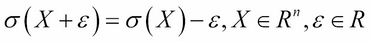
- Translation invariance: Adding a constant value to the portfolio decreases the risk by the same amount. See the following formula:
If the standard deviation is not a reliable risk measure, then what can we use? This question popped up at J.P. Morgan by CEO Dennis Weatherstone in the early 1990s. He called the firm's departments for the famous 4:15 report, in which they aggregated the so-called values at risk 15 minutes before the market closed. The CEO wanted an aggregated measure that showed what amount the firm might lose in the next trading day. As this cannot be calculated with full certainty, especially in the light of the 1987 Black Monday, the analysts added a probability of 95 percent.
The figure that shows what a position might lose in a specified time period with a specified probability (significance level) is called the Value at Risk (VaR). Although it is quite new, it is widely used both by risk departments and financial regulators. There are several ways to calculate value at risk, which can be categorized into three different methods. Under the analytical VaR calculation, we assume that we know the probability distribution of the underlying asset or return. If we do not want to make such assumptions, we can use the historical VaR calculation using the returns or asset values realized in the past. In this case, the implicit assumption is that the past development of the given instrument is a good estimator for the future distribution. If we would like to use a more complex distribution function that is hard to tackle by analytics, a Monte-Carlo simulation could be the best choice to calculate VaR. This can be used by either assuming an analytical distribution of the instrument or by using past values. The latter is called historic simulation.
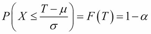
When calculating Value at Risk (VaR) in an analytical approach, we need to assume that the return of a financial instrument follows a certain mathematical probability distribution. The normal distribution is used most commonly; that is why we usually call it the delta-normal method for VaR calculation. Mathematically, X ~ N (μ,σ), where μ and σ are the mean and the standard deviation parameters of the distribution. To calculate the value at risk, we need to find a threshold (T) that has the ability that the probability of all data bigger than this is α (α is the level of significance that can be 95 percent, 99 percent, 99.9 percent, and so on). Using the standard normal cumulative distribution for function F:
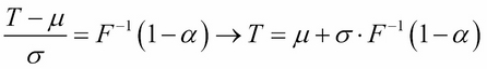
This indicates that we need to apply the inverse cumulative distribution function to 1- α:
Although we do not know the closed mathematical formula of neither the cumulative function of normal distribution nor its inverse, we can solve this by using a computer.
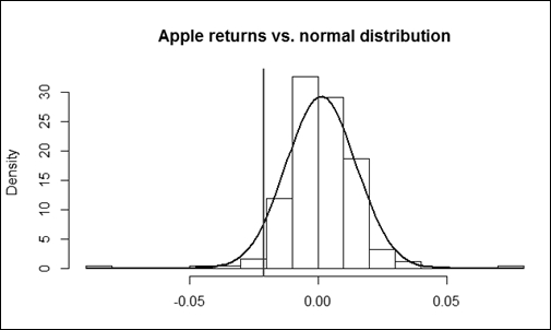
We use R to calculate the 95 percent, 1 day VaR of the Apple stocks using the delta normal method, based on a two-year dataset. The estimated mean and standard deviation of Apple returns are 0.13 percent and 1.36 percent.
The following code calculates that VaR for Apple stocks:
Apple <- read.table("Apple.csv", header = T, sep = ";")
r <- log(head(Apple$Price,-1)/tail(Apple$Price,-1))
m <- mean(r)
s <- sd(r)
VaR1 <- -qnorm(0.05, m, s)
print(VaR1)
[1] 0.02110003
The threshold, which is equal to the VaR if we apply it to the returns, can be seen in the following formula. Note that we always take the absolute value of the result, as VaR is interpreted as a positive number:
The VaR (95 percent, 1 day) is 2.11 percent. This means that it has 95 percent probability that Apple shares will not lose more than 2.11 percent in one day. We can also interpret this with an opposite approach. An Apple share will only lose more than 2.11 percent in one day with 5 percent probability.
The chart shown in the following figure depicts the actual distribution of Apple returns with the historic value at risk on it:
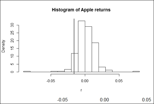
The simplest way of calculating the value at risk is by using the historical approach. Here, we assume that the past distribution of the financial instrument's return represents the future too. Therefore, we need to find the threshold above which the α portion of the values can be found. In statistics, this is called the percentile. If we use a VaR with a 95- percent level of significance, for instance, then it will imply the lower fifth percentile of the dataset. The following code shows how to calculate the percentile in R:
VaR2 <- -quantile(r, 0.05)print(VaR2)
        5%
0.01574694
Applying this to the Apple shares, we get a lower fifth percentile of 1.57 percent. The value at risk is the absolute value of this percentile. Therefore, we can either say that it has only 5 percent probability that Apple shares lose more than 1.57 percent in a day, or the stock will lose less than 1.57 percent with 95 percent likelihood.
The most sophisticated approach to calculate the value at risk is the Monte-Carlo simulation. However, it is only worth using if other methods cannot be used. These reasons can be the complexity of the problem or the assumption of a difficult probability distribution. Nevertheless, this is the best method to show the powerful capabilities of R that can support risk management.
A Monte-Carlo simulation can be used in many different fields of finance and other sciences as well. The basic approach is to set up a model and to assume an analytic distribution of the exogenous variable The next step is to randomly generate the input data to the model in accordance with the assumed distribution. Then, the outcomes are collected and used to gather the result and draw the conclusion. When the simulated output data is ready, we can follow the same procedure as we would do if we used the historical approach.
Using a 10,000 step Monte-Carlo simulation to calculate the value at risk of Apple shares may seem to be an overkill, but it serves for the demonstration. The related R code is shown here:
sim_norm_return <- rnorm(10000, m, s)
VaR3 <- -quantile(sim_norm_return, 0.05)
print(VaR3)
        5%
0.02128257
We get a result of 2.06 percent for the value at risk as a lower fifth percentile of the simulated returns. This is very close to the 2.11 percent estimated with the delta-normal method, which is not a coincidence. The basic assumption that the yield follows a normal distribution is the same; thus, the minor difference is only a result of the randomness of the simulation. The more steps the simulation takes, the closer the result is to the delta-normal estimation.
A modification of the Monte-Carlo method is the historical simulation when the assumed distribution is based on the past data of the financial instrument. The generation of the data here is not based on an analytical mathematical function but the historical values are selected randomly, preferably via an independent identical distribution method.
We also use a 10,000 element simulation for the Apple stock returns. In order to select the values from the past randomly, we assign numbers to them. The next step is to simulate a random integer between 1 and 251 (the number of historic data) and then use a function to find the associated yield. The R code can be seen here:
sim_return <- r[ceiling(runif(10000)*251)]
VaR4 <- -quantile(sim_return, 0.05)
print(VaR4)
        5%
0.01578806
The result for the VaR is 1.58 percent, which is not surprisingly close to the value derived from the original historic method.
Nowadays, value at risk is a common measure for risk in many fields of finance. However, in general, it still does not fulfill the criteria of a coherent risk measure as it fails to meet sub-additivity. In other words, it might discourage diversification in certain cases. However, if we assume an elliptically distributed function for the returns, the VaR proves to be a coherent risk measure. This essentially means that the normal distribution suits the estimation of VaR perfectly. The only problem is that the stock returns in real life are rather leptokurtic (heavy-tailed) compared to the Gaussian curve as it is experienced as a stylized fact of finance.
In other words, the stocks in real life tend to show more extreme losses and profits than it would be explained by the normal distribution. Therefore, a developed analysis of risk assumes more complex distributions to cope with the heavy-tailed stock returns, the heteroskedasticity, and other imperfections of the real-life yields.
The use of Expected Shortfall (ES) is also included in the developed analysis of risk, which is, in fact, a coherent risk measure, no matter what distribution we assume. The expected shortfall concentrates on the tail of the distribution. It measures the expected value of the distribution beyond the value at risk. In other words, the expected shortfall at α significance level is the expected value of the worst α percent of the cases. Mathematically, ![]() .
.
Here, VaRγ is the value at risk of the distribution of returns.
Sometimes, an expected shortfall is called conditional value at risk (CVaR). However, the two terminologies do not exactly mean the same thing; they can be used as synonyms if continuous distribution functions are used for the risk analysis. Although R is capable of dealing with such complex issues as the expected shortfall, it goes beyond the goals of this book. For further information on this topic, see the work of Acerbi, C.; Tasche, D. (2002).