
This chapter introduces the usage of R for commercial bank asset and liability management (ALM) purposes. The ALM function in a bank is traditionally associated with interest rate risk and liquidity risk management of banking book positions. Both of the interest rate positioning and liquidity risk management require the modeling of banking products. Nowadays, professional ALM units use complex Enterprise Risk Management (ERM) frameworks, which are able to incorporate the management of all risk types and provide an adequate tool for ALM to steer the balance sheet. Our general objective is to set up a simplified framework of ALM to illustrate the use of R for certain ALM tasks. These tasks are based on the interest rate and liquidity risk management and the modeling of non-maturing accounts.
This chapter is structured as follows. We start with the data-preparation process of ALM analysis. The process of planning and measurement needs special information about the banking book, market conditions, and the business strategy. This part establishes a data-management tool that consists of the major input datasets, and extracts data into the form that we use in the rest of this chapter.
Next, we will be dealing with the measurement of the interest rate risk. There are two common approaches in the banking industry to quantify interest rate risk in the banking book. Simpler techniques use repricing gap table analysis to manage the interest rate risk exposure and calculate parallel yield curve shocks to forecast the net interest income (NII) and calculate the market value of equity (MVoE). More advanced methods use dynamic simulation of balance sheets and stochastic simulation of interest rate development. Choosing which tool to use depends on the targets and the balance sheet structure.
For example, a savings bank (with client term deposits on the liability side and fix bond investments on the asset side) focuses on its market value of equity risk, while a corporate bank (with floating interest position) concentrates on the net interest income risk. We illustrate how to efficiently provide a repricing gap table and net interest income forecasts with R.
Our third topic is related to the liquidity risk. We define three types of liquidity risks: structural, funding, and contingency risks. Structural liquidity risks arise from the different contractual maturities on the asset and liability side. Commercial banks usually collect short-term client deposits and place the acquired funding into long-term client loans. As a result, the bank is exposed to a roll-over risk on the liability side as it is uncertain how much of the maturing short term client funding will be rolled over, which endangers the solvency of the bank. Funding liquidity risks occur during the roll-overs; it refers to the uncertainty of the cost of renewed funding. In ordinary course of business, even though a bank can roll over its maturing interbank deposits, the cost of the deals highly depends on the available liquidity on the market. Contingency risk refers to the behavior of the clients in unforeseen scenarios. For example, a contingency risk appears as sudden withdrawals of term deposits or premature repayments among the client loans. While ALM appropriately handles the structural and funding liquidity risks by regulating bank positions, contingency liquidity risks can only be hedged by buffering liquid assets. We show how to build up liquidity gap tables and forecast net financing needs.
In the last section of this chapter, we will concentrate on the modeling of non-maturing products. Client products can be classified by their maturity structure and interest rate behavior. Examples of typical non-maturing liability products are on-demand deposits and savings accounts without any notice period of withdrawal. The clients can withdraw their money at any time, while the bank has the right to modify the offered interest rate. On the asset side, overdrafts and credit cards show quite similar characteristics. The complex models of non-maturing products make the work of ALM quite challenging. Practically, the modeling of non-maturing products means the mapping of the cash-flow profiles, estimating the interest rate elasticity of the demand, and analyzing the liquidity-related costs in the internal funds transfer pricing (FTP) system. Here, we demonstrate how to measure the interest sensitivity of the non-maturing deposits.
Complex ERM software are essential tools in the banking industry to quantify the net interest income and the market value of equity risks, and to prepare reports particularly on the asset and liability portfolio, the re-pricing gaps, and the liquidity positions. We set up a simplified simulation and reporting environment using R, which reproduces the key features of the commercially used ALM software solutions.
Typical ALM data processes follow the so-called extract, transform, and load (ETL) logic.
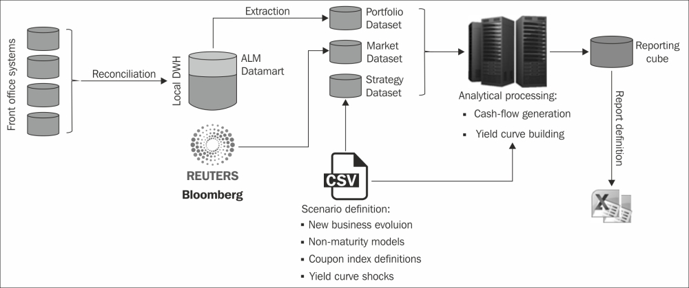
Extraction, which is the first phase, means that the bank has already collected the deal-level and account-based source data from the local data warehouse (DWH), the mid-office, the controlling or the accounting systems. The source data of the total balance sheet (here called a portfolio) is also extracted in order to save calculation time, memory and storage space. Moreover, single deal-level data is aggregated by the given dimensions (for example, by currency denomination, interest behavior, amortization structure, and so on). Market data (such as yield curves, market prices, and volatility surfaces) is also prepared in a raw dataset. The next step is to set the simulation parameters (for example, yield curve shocks and volume increments of the renewed business), in which we call strategy. For the sake of simplicity, here we reduce this strategy to keep the existing portfolio therefore the balance sheet remains the same forecasted period.
At the stage of transformation, the portfolio, market, and strategy datasets are combined and used for further analysis, and are transformed into new structures. In our terms, this means that the cash-flow table is generated by using the portfolio and market descriptors, and it is converted into a narrow data form.
At the time of loading, the results are written into a reporting table. Usually, users can define what dimensions of the portfolio and values of risk measures should be loaded into the result database. We will show how liquidity risk and interest rate risk can be measured and documented in the following sections.
We call the data source that lists the balance sheet items "portfolios". Market data (such as yield curves, market prices, and volatility surfaces) is also prepared in a raw dataset. Let's import our initial datasets into R. First of all, we need to download the datasets and the functions to be used in this chapter from the link of Packt Publishing. Now, let's import the sample portfolio and market datasets that are stored in standard csv format in a local folder that is used in the code as follows:
portfolio <- read.csv("portfolio.csv")
market <- read.csv("market.csv")
The selected datasets contain dates that have to be converted into the appropriate format. We transform the date formats with the as.Date function:
portfolio$issue <- as.Date(portfolio$issue, format = "%m/%d/%Y")
portfolio$maturity <- as.Date(portfolio$maturity, format = "%m/%d/%Y")
market$date <- as.Date(market$date, format = "%m/%d/%Y")
Print the first few rows of the imported portfolio dataset with the head(portfolio) command. It results the following output:
head(portfolio)
  id account                        account_name volume
1  1    cb_1 Cash and balances with central bank    930
2  2   mmp_1             Money market placements   1404
3  3   mmp_1             Money market placements    996
4  4    cl_1                     Corporate loans    515
5  5    cl_1                     Corporate loans    655
6  6    cl_1                     Corporate loans    560
  ir_binding reprice_freq spread      issue   maturity
1        FIX           NA      5 2014-09-30 2014-10-01
2        FIX           NA      7 2014-08-30 2014-11-30
3        FIX           NA     10 2014-06-15 2014-12-15
4      LIBOR            3    301 2014-05-15 2016-04-15
5      LIBOR            6    414 2014-04-15 2016-04-15
6      LIBOR            3    345 2014-03-15 2018-02-15
  repayment payment_freq yieldcurve
1    BULLET            1      EUR01
2    BULLET            1      EUR01
3    BULLET            1      EUR01
4    LINEAR            3      EUR01
5    LINEAR            6      EUR01
6    LINEAR            3      EUR01
The columns of this data frame refer to the identification number (the number of the row), the account type, and the product characteristics. The first three columns represent the product identifier, the account identifier (or the short name), and the long name of the account. Using the levels function, we can easily list the type of accounts that are related to the typical commercial bank products or balance sheet items:
levels(portfolio$account_name)
 [1] "Available for sale portfolio"
 [2] "Cash and balances with central bank"
 [3] "Corporate loans"
 [4] "Corporate sight deposit"
 [5] "Corporate term deposit"
 [6] "Money market placements"
 [7] "Other non-interest bearing assets"
 [8] "Other non-interest bearing liabilities"
 [9] "Own issues"
[10] "Repurchase agreements"
[11] "Retail overdrafts"
[12] "Retail residential mortgage"
[13] "Retail sight deposit"
[14] "Retail term deposit"
[15] "Unsecured money market funding"
The portfolio dataset also contains the notional volume in EUR, the type of the interest binding (FIX or LIBOR), the repricing frequency of the account in the number of months (if the interest binding is LIBOR), and the spread component of the interest rate in basis points. Furthermore, other columns describe the cash-flow structure of the products. The columns are issue date (this is the first repricing day), maturity date, the type of principal repayment structure (bullet, linear, or annuity), and the repayment frequency in number of months. The last column stores the identifier of the interest rate curve, what we use for the calculation of future floating rate payments.
Actual interest rates are stored in the market dataset. Let's list some of the first few rows to check the content:
head(market)
   type       date       rate comment
1 EUR01 2014-09-01  0.3000000      1M
2 EUR01 2014-12-01  0.3362558      3M
3 EUR01 2015-03-01 -2.3536463      6M
4 EUR01 2015-09-01 -5.6918763      1Y
5 EUR01 2016-09-01 -5.6541774      2Y
6 EUR01 2017-09-01  1.0159576      3Y
The first column indicates the yield curve type (for example, yields are from the bond market or the interbank market). The type column has to be the same as in portfolio to connect the two datasets. The date column shows the maturity of the current rate, and rate indicates the value of the rate in basis points. As you can see, the yield curve is very unusual at this time as there are negative yield curve points for certain tenors. The last column stores the label of the yield curve tenor.
The datasets reflect the current state of the bank portfolio and the current market environment. The actual date is September 30, 2014 in our analysis. Let's declare it as a date variable called NOW:
NOW <- as.Date("09/30/2014", format = "%m/%d/%Y")
Now, we finished the preparation of our source data. This is a sample dataset created by the authors for illustrative purposes, and demonstrates the simplified version of a hypothetical commercial bank balance sheet structure.
After we import the static data of our balance sheet and the current yield curve, we use this information to generate the total cash-flow of the bank. First, we calculate the floating interest rates using the forward yield curve; after that, we can generate separately the principal and interest cash-flows. For this purpose, we predefine the basic functions to calculate principal cash-flows based on payment frequencies and to extract floating interest rates for variable interest rate products. This script is also available on the link provided by Packt Publishing.
Copy it into the local folder and run the script of the predefined functions from the working directory.
source("bankALM.R")
This source file loads the xts, zoo, YieldCurve, reshape, and car packages, and if necessary, it installs these required packages. Let's take a look at the most important functions we use from this script file. The cf function generates a predefined cash-flow structure. For example, generating a bullet payment structure loan with the nominal value of EUR 100, a maturity of three years, and a fixed interest rate of 10 percent looks like this:
cf(rate = 0.10, maturity = 3, volume = 100, type = "BULLET")
$cashflow
[1]  10  10 110
$interest
[1] 10 10 10
$capital
[1]   0   0 100
$remaining
[1] 100 100   0
The function provides the entire cash-flow, the interest and capital repayment structure, and the value of the remaining capital in each period. The get.yieldcurve.spot function provides a fitted spot yield curve on a certain sequence of dates. This function uses the YieldCurve package, what we have already loaded before. Let's define a test variable of dates, as follows:
test.date <- seq(from = as.Date("09/30/2015", format = "%m/%d/%Y"), to = as.Date("09/30/2035", format = "%m/%d/%Y") , by = "1 year")
Get and plot the fitted spot yields on the specified dates using the market data:
get.yieldcurve.spot(market, test.date, type = "EUR01", now = NOW, showplot = TRUE)
The following screenshot is the result of the preceding command:
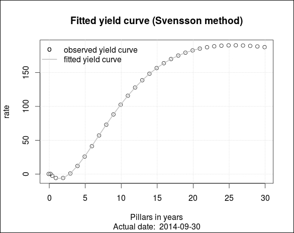
The preceding graph draws the observed yield curve (points) and the fitted yield curve (line). Looking at the get.yieldcurve.forward and get.floating functions, we see that both of them use the repricing date of the balance sheet product. The following example generates a sequence of repricing dates for a period of 20 timepoints.
test.reprice.date <- test.date[seq(from = 1,to = 20, by = 2)]
Extract the forward yield curve using the market data:
test.forward <- get.yieldcurve.forward(market, test.reprice.date,type = "EUR01", now = NOW)
Now, let's generate the floating rates and illustrate the difference between the forward curve and the test.floating variable by setting the showplot option to TRUE.
test.floating<-get.floating(test.date, test.reprice.date, market, type = "EUR01", now = NOW, shoplot = TRUE)
The following screenshot gives the output for the preceding command:
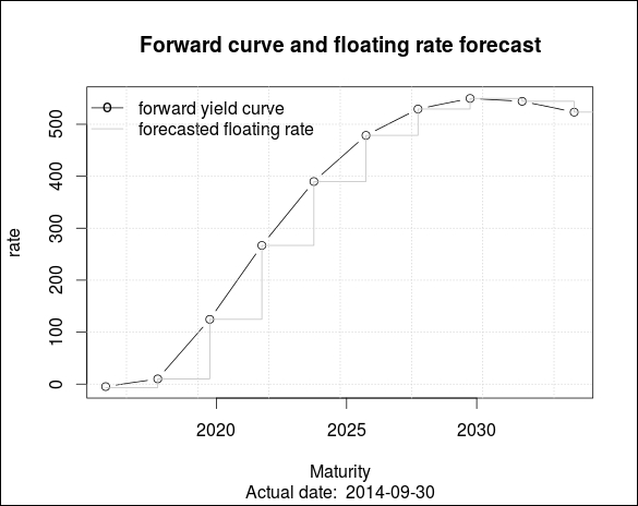
As you can see, the floating rate forecast consists of a step-wise function. For pricing purposes, the floating rate is substituted by the actual forward rate; however, the floating rate is only updated at the time of repricing.
In the next steps, we will demonstrate the cash-flow table that we produce from our portfolio and market datasets. The cf.table function calls the functions detailed earlier and provides a cash-flow of the exact product, which has the id identification number. In the portfolio dataset, identification numbers have to be integers, and they have to be in an increasing order. Practically, each of them should be the line number of the given row. Let's generate the cash-flow of all products:
cashflow.table <- do.call(rbind, lapply(1:NROW(portfolio), function(i) cf.table(portfolio, market, now = NOW, id = i)))
As the portfolio dataset contains 147 products, the running of this code might take a few (10-60) seconds. When we are ready, let's check the result that shows the first few lines:
head(cashflow.table)
  id account       date        cf interest capital remaining
1  1    cb_1 2014-10-01  930.0388  0.03875     930         0
2  2   mmp_1 2014-10-30    0.0819  0.08190       0      1404
3  2   mmp_1 2014-11-30 1404.0819  0.08190    1404         0
4  3   mmp_1 2014-10-15    0.0830  0.08300       0       996
5  3   mmp_1 2014-11-15    0.0830  0.08300       0       996
6  3   mmp_1 2014-12-15  996.0830  0.08300     996         0
Now we are done with the creation of the cash-flow table. We can also calculate the present value of the products and, the market value of the equity of the bank. Let's run the pv.table function in the following loop:
presentvalue.table <- do.call(rbind, lapply(1:NROW(portfolio), function (i) pv.table(cashflow.table[cashflow.table$id == portfolio$id[i],], market, now = NOW)))
Print the initial rows of the table to check the results:
head(presentvalue.table)
  id account       date presentvalue
1  1    cb_1 2014-09-30     930.0384
2  2   mmp_1 2014-09-30    1404.1830
3  3   mmp_1 2014-09-30     996.2754
4  4    cl_1 2014-09-30     530.7143
5  5    cl_1 2014-09-30     689.1311
6  6    cl_1 2014-09-30     596.3629
The results might differ slightly because the Svensson method may produce different outputs. To get the market value of equity, we need to add the present values.
sum(presentvalue.table$presentvalue)
[1] 14021.19
The cash-flow table handles liabilities as negative assets; hence, adding up all the items provides us with the appropriate results.