
The best way to understand the role of a bank from a systemic point of view is to simulate the effects of its default. We can get this way the most precise results on a bank's systemic importance. Usually, the main problem with these methods is its data need. The main characteristics of individual institutions (for example, capital buffers or size) are not enough for this kind of exercise. We also have to precisely know its exposures to other banks through financial markets since the most important contagious channels are financial markets.
In this section, we will show a simple method to identify systemic importance of a financial institution. To make it as simple as possible, we have to make some assumptions:
- We will investigate the effect of idiosyncratic defaults. After the default, all the contagious effects go through the network abruptly.
- Since all the effects go through abruptly, there won't be any adjustment procedure by banks.
- LGD is constant for all the banks. There are models that take into account the fact that the LGD can change from bank to bank (for example, Eisenberg and Noe, 2001), but this would make our model too complicated.
- We don't take into account the length of the legal procedure after the default. In practice, it should be considered in the LGD.
As we mentioned in the data section, we will need three datasets. First, we need the matrix that contains the exposures of the banks to each other on the interbank deposit market. Since these transactions are not collateralized, the potential losses are the biggest on this market. Second, we need the size of the capital buffers for each bank. The possibility of contagious effects can be significantly mitigated by a high capital buffer. For this reason, it is always important to check what can be considered as a capital buffer. Our opinion is that only the capital that exceeds the regulatory minimum should be taken into account in this exercise to be as prudent as possible. Third, we need the size of each bank. To evaluate the effect of one bank's default, we need the size of infected banks. In our example, we use the balance sheet total, but other measures can be used as well. The chosen measure has to proxy the effects on the real economy (for example, it can be the size of the corporate loan portfolio or the stock of deposits and so on).
As a first step, we randomly choose a bank (any of them, since we will do this for every bank), and we assume that it is defaulted after an idiosyncratic shock. The matrix contains all the information about the banks that were lending to this one. Wij is the size of the loan that was borrowed by bank j from bank i. L is the LGD, that is, the size of the loss proportional to the exposure. When the following inequality stays, that is, the loss of bank i from the default of bank j exceeds the capital buffer of bank i, bank i has to be considered as defaulted.
As a result, we get all those partner banks of bank j, which defaulted after the collapse of bank j. We make the first step in case of the partner banks of all the newly defaulted banks. We continue this simulation until we reach an equilibrium situation where there are no new defaults.
We make this simulation for every bank, that is, we try to find out which banks will default after their collapse due to contagious effects. Finally, we aggregate the balance sheet total of the defaulted banks in each case. Our final result will then be a list that contains the potential effect of the default of each bank based on the market share of the affected banks.
In this section, we will show how to implement this simulation technique in R. We will present the whole code as before. Some parts of the code were also used in the core-periphery distinction as well, so we won't give a detailed explanation for them.
In the first few rows, we set some basic information. There are two rows where explanation is needed. First, we set the value of the LGD. As we will see later, it is important to make our examinations by using different LGDs since our simulation is sensitive on the level of the LGD. The value can be anything from 0 to 1. Second, those algorithms that plot the network use a random number generator. The Set.seed command sets the initial value of the random number generator to ensure that we get graphs with the same outlook.
LGD = 0.65
set.seed(3052343)
library(igraph)
In the next part of the code, we load the data, which will be used in the model, namely the matrix of the network (mtx.csv), the vector of the capital buffer (puf.csv), and the vector of the bank's size (sizes.csv).
adj_mtx <-  read.table("mtx.csv", header = T, sep = ";")
node_w <-   read.table("puf.csv", header = T, sep = ";")
node_s <- read.table("sizes.csv", header = T, sep = ";")
adj_mtx <- as.matrix(adj_mtx)
adj_mtx[is.na(adj_mtx)] <- 0
During the simulation, the adjacency matrix is not enough, contrary to the core-periphery distinction. We need the weighted matrix G.
G <- graph.adjacency((adj_mtx ), weighted = TRUE)
The next step is technical rather than essential, but it helps to avoid any mistakes later. V is the set of the graph's nodes. We put together all the relevant information about each node, that is, in which step it has defaulted (non-defaulted banks get 0), the capital buffer, and the size.
V(G)$default <- 0
V(G)$capital <- as.numeric(as.character(node_w[,2]))
V(G)$size <- as.numeric(as.character(node_s[,2]))
Then, we can easily plot the network. We have used this command to create Figure 13.2. Of course, it is not essential for the simulation.
plot(G, layout = layout.kamada.kawai(G), edge.arrow.size=0.3, vertex.size = 10, vertex.label.cex = .75)
As we mentioned, our goal is to get a list of banks and the effect of their collapse on the banking system. However, it is also worth seeing the process of the contagion in every case. For this reason, we use a function that can generate a chart about it. The sim function has four attributes: G is the weighted graph, the starting node that is the first defaulted bank, the LGD, and finally a variable to switch the plotting of the graph on or off. The last two attributes have a default value, but of course, we can give them a different value during each run. We also set different colors for each node depending on in which step it has defaulted.
sim <- function(G, starting_node, l = 0.85, drawimage = TRUE){
node_color <- function(n,m) c(rgb(0,0.7,0),rainbow(m))[n+1]
We create a variable that helps us know whether the contagion has stopped or not. We also create a list that contains the defaulted banks. The jth component of the list contains all the banks collapsed in the jth step.
stop_ <- FALSE
j <- 1
default <- list(starting_node)
The next part is the essence of the whole code. We start a while loop and check whether the contagion goes on or not. Initially, it goes on for sure. We set the default attribute to j for those banks that collapse in the jth step.
Then, in a for loop, we take all the banks that have connections with bank i, and deduct exposure*LGD from their capital. The banks that default after this will be on the default list. Then, we start again with the exposure to the newly defaulted banks and continue with it until there won't be any new defaults.
while(!stop_){
V(G)$default[default[[j]]] <- j
j <- j + 1; stop_ <- TRUE
for( i in default[[j-1]]){V(G)$capital <- V(G)$capital - l*G[,i]}
default[[j]] = setdiff((1:33)[V(G)$capital < 0], unlist(default));
if( length( default[[j]] ) > 0) stop_ <- FALSE
}
When drawimage is equal to T in the sim function, the code will plot the network. The color of each node depends on the time of default, as we mentioned before. Banks that defaulted later get a lighter color, and those that have not defaulted get a green color.
if(drawimage) plot(G, layout = layout.kamada.kawai(G), edge.arrow.size=0.3, vertex.size = 12.5, vertex.color = node_color(V(G)$default, 4*length(default)), vertex.label.cex = .75)
Then, we count the proportion of the collapsed banks that are contained in the default list.
sum(V(G)$size[unlist(default)])/sum(V(G)$size)}
Using the function sapply, we can run the same function for every component of a vector and collect the results in a list.
result <- sapply(1:33, function(j) sim(G,j,LGD, FALSE))
Finally, we make a barplot that contains the result of every bank in the system. This chart makes it possible to decide about systemic importance.
dev.new(width=15,height=10)
v <- barplot(result, names.arg = V(G)$name, cex.names = 0.5, ylim = c(0,1.1))
text(v, result, labels = paste(100*round(result, 2), "%", sep = ""), pos = 3, cex = 0.65)
Our main question during this exercise was: which banks were the systemically important financial institutions. After running the code we have shown in the last subchapter we get an exact answer on our question. The chart pops up after the run summarizes the main results of the simulation. The horizontal axis has the codes of the banks, while the vertical axis has the proportion of the banking system affected by the idiosyncratic shock. For example, in figure 13.6., 76 percent at X3 means that if bank number 3 defaults due to an idiosyncratic shock, 76 percent of the whole banking system will default as a result of contagion. It is a matter of decision to set a level above which a bank has to be considered as systemically important. In this example, it is easy to distinguish between institutions that have to be taken as SIFIs and those that have minor relevance for the system. According to Figure 13.6., 10 banks (with codes 3, 7, 12, 13, 15, 18, 19, 21, 24, and 28) can be considered as systemically important.
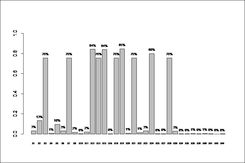
Figure 13.6: Proportion of the banking system based on the balance sheet total affected by the idiosyncratic shock LGD = 0.65
It is important to mention that the result is dependent on the LGD parameter, which has to be set in the code. In this first run, the LGD was set to 65 percent, but it can differ significantly in different cases. For example, if the LGD is 90 percent, the result will be much worse. Five more banks (their codes are 2, 8, 11, 16, and 20) will also have a significantly negative effect on the banking system in the case of an idiosyncratic shock. However, with a much lower LGD, the result will also be milder. For example, if the LGD level is set to 30 percent bank number 13 will have the biggest effect on the banking system. However, by comparing this to the former examples, this effect will be very limited. 36 percent of the banking system will default in this case. Using the 30 percent LGD level, only 4 banks will have more than 10 percent effect on the system (Figure 13.7).
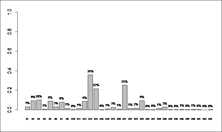
Figure 13.7.: Proportion of the banking system based on balance sheet total affected by the idiosyncratic shock LGD = 0.3
This R code is also able to show us the process of contagion. By running the sim function, it is possible to find out which banks are affected directly by the default of an examined bank and which banks are affected in the second or third or later step of the simulation. For example, if we want to know what happens when bank 15 defaults, we write in the R console the following command: sim(G, 13, 0.65), where G is the matrix, 13 is the ordinal number of bank number 15, and 65 percent is the LGD. As a result, we get figure 13.8. We sign the bank that launches the contagion with a red color. Orange is the color of those institutions that are affected directly by the idiosyncratic shock of bank number 15. Then, when the color is lighter, the bank is affected later. Finally, banks with green nodes are the survivors. LGD was set at 65 percent in this example. It can be seen that the collapse of bank number 15 will result directly the default of five other banks (with codes 8, 18, 20, 21, and 36). Then, with the default of these banks, many more will also lose their capital. At the end, more than 80 percent of the banking system will be in default.
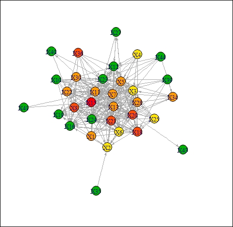
Figure 13.8: The contagion process after the default of bank number 15
It has to be emphasized that with this simulation method, not only were the interbank exposures taken into account but also the size of the main partners and the capital buffer of them. In this case, systemic importance can be a result of undercapitalized partners. Or on the contrary, it is possible that a bank with many partners and borrowed money won't have any negative effect on the market since its direct partners have a high enough capital buffer. Bank number 20 is a good example of this. In the core-periphery decomposition, it is definitely in the core. However, when we run the sim function with a 65 percent LGD, the result will be very different. Figure 13.9 presents that none of the other banks will default after its idiosyncratic shock.
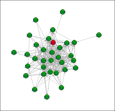
Figure 13.9: Contagion process after the default of bank number 20