
Like the Vasicek model, the Cox-Ingersoll-Ross model (Cox at al., 1985), which is often cited as the CIR model, is a continuous, affine, one-factor stochastic interest rate model. In this model, the instantaneous interest rate dynamics are given by the following stochastic differential equation:
Here, α, β, and σ are positive constants, rt is the interest rate, t is the time, and Wt denotes the standard Wiener process. It is easy to see that the drift component is the same as in the Vasicek model; hence, the interest rate follows a mean-reverting process again, β is the long-run average, and α is the rate of adjustment. The difference is that the volatility term is not constant but is proportional to the square root of the interest rate level. This 'small' difference has dramatic consequences regarding the probability distribution of the future short rates. In the CIR model, the interest rate has non-central chi-squared distribution, with the following density function (f):
Here, ![]() ,
, ![]() , and
, and 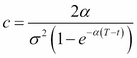 .
.
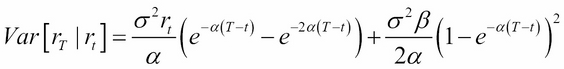
Here, ![]() denotes the probability density function of the chi-squared distribution with n degrees of freedom and m denoting the non-centrality parameter. As the expected value and the variance of such a random variable is n+m and 2(n+2m) respectively, we have the following moments for the interest rate:
denotes the probability density function of the chi-squared distribution with n degrees of freedom and m denoting the non-centrality parameter. As the expected value and the variance of such a random variable is n+m and 2(n+2m) respectively, we have the following moments for the interest rate:

We might observe that the conditional expected value is exactly the same as in the Vasicek model. It is important to notice that the short rate, as a normally distributed variable, might become negative in the Vasicek model, but this cannot happen in the CIR model.
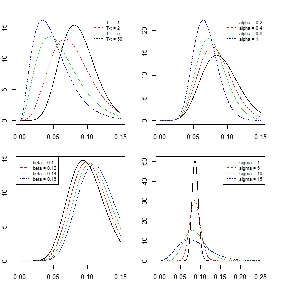
Like in the case of the Vasicek model, we can see how the coefficients determine the shape of the probability density function if we plot it with different parameter sets. The following code does this job by comparing the probability density functions under various parameter specifications:
CIR_pdf = function(x, alpha, beta, sigma, delta_T, r0 = 0.1){
  q = (2*alpha*beta)/(sigma^2) - 1
  c = (2*alpha)/(sigma^2*(1-exp(-alpha*delta_T)))
  u = c*r0*exp(-alpha*delta_T)
  2*c*dchisq(2*c*x, 2*q+2, ncp = 2*u)
              }

x <- seq(0, 0.15, length = 1000)
y <- sapply(c(1, 2, 5, 50), function(delta_T)
       CIR_pdf(x, .3, 0.05,0.1,delta_T))

par(mar = c(2,2,2,2), mfrow = c(2,2))
matplot(x, y, type = "l",ylab ="",xlab = "")
legend("topright", c("T-t = 1", "T-t = 2", "T-t = 5", "T-t = 50"), lty = 1:4, col = 1:4, cex = 0.7)

y <- sapply(c(.2, .4, .6, 1), function(alpha)
       CIR_pdf(x, alpha, 0.05,0.1,1))
  matplot(x, y, type = "l",ylab ="",xlab = "")
legend("topright", c("alpha = 0.2", "alpha = 0.4", "alpha = 0.6", "alpha = 1"), lty = 1:4, col = 1:4, cex = 0.7)

y <- sapply(c(.1, .12, .14, .16), function(beta)
       CIR_pdf(x, .3, beta,0.1,1))

matplot(x, y, type = "l",ylab ="",xlab = "")
legend("topleft", c("beta = 0.1", "beta = 0.12", "beta = 0.14", "beta = 0.16"), lty = 1:4, col = 1:4, cex = 0.7)

x <- seq(0, 0.25, length = 1000)
y <- sapply(c(.03, .05, .1, .15), function(sigma)
       CIR_pdf(x, .3, 0.05,sigma,1))

matplot(x, y, type = "l",ylab ="",xlab = "")
legend("topright", c("sigma = 1", "sigma = 5", "sigma = 10", "sigma = 15"), lty = 1:4, col = 1:4, cex = 0.7)
Here, we can see the result. We come to the same conclusion as we did in the case of the Vasicek model, except that here, β changes the shape of the density function and not just shifts it.
Pricing a zero-coupon bond in the CIR model yields the following formula (see, for example, Cairns [2004]):
Here, 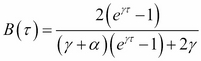 ,
, 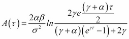 , and
, and ![]() .
.
Determining the yield curve from the bond prices is exactly the same as in the Vasicek model.