
Interbank markets are tiered and operate in a hierarchical fashion. It is a well-known characteristic of these markets that many banks are dealing with only a small number of big institutions, while these big institutions are acting like intermediaries or money-center banks. These big institutions are considered to be the core of the network, and the others are the periphery.
Many papers focused on this characteristic of real-world networks. For example, Borgatti and Everett (1999) examined this phenomenon on a network made of citation data, and found three journals to be the members of the core. Craig and von Peter (2010) used this core/periphery structure for the German interbank market. Their findings suggest that bank-specific features help to explain how banks position themselves in the interbank market. There is a strong correlation between the size and position in the network. As tiering is not random but behavioral, there are economic reasons (for example, fixed costs) why the banking system organizes itself around a core of money-center banks. This finding also implies that coreness can be a good measure of systemic importance.
A perfect core-periphery structure of a network can be presented easily by the matrix in Figure 13.3. Core banks are in the upper-left corner of the matrix. All of these banks are connected to each other. They can be considered as intermediaries. They are responsible for the stability of the market, and other banks are connected to each other through these core institutions. In the lower-right corner, there are periphery banks. They have no connection with other periphery institutions. They are only connected to the core as shown in the following screenshot:
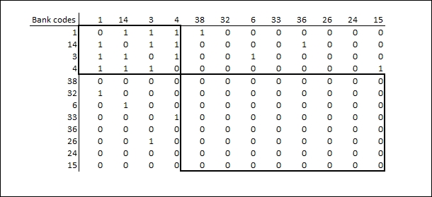
Figure 13.4: The adjacency matrix in a core periphery structure
Craig and von Peter (2010) also suggest that not only the core-core or the periphery-periphery part of the matrix is important but the core-periphery part is important as well (the upper-right and the lower-left part). They emphasize that all of the core banks should have at least one connection with a periphery institution. This characteristic means that this periphery bank has no other possibility to be on this market but through a core bank. Although it is an important issue, we think that due to possible contagious effects, being a core bank in itself can result in systemic importance.
In many cases, it is impossible to get pure core/periphery decomposition in the case of real-world networks. This is true especially when we also have requirements for the core-periphery part of the matrix. For this reason, in the first step, we will try to solve the maximum clique problem (for example, by using the Bron-Kerbosch algorithm, Bron and Kerbosch 1973), and then, in the second step, we will choose the result with the lowest average degree in the periphery-periphery part. There are many other different methods to make a core-periphery decomposition. Due to its simplicity, we have chosen this one.
In this subsection, we show how to program the core-periphery decomposition. We will cover all the relevant information, from downloading essential R packages to loading the data set, and from the decomposition itself to the visualization of the results. We will show the code in small parts, and will give a detailed explanation on each of them.
We set the library that we will use during the simulation. The code will look for the input data files in this library. We download an R package igraph, which is an important tool in the visualization of financial networks. Of course, after the first run of this code, this row might be deleted since the installation process should not be repeated again. Finally, after the installation, the package should also be loaded first to the current R session.
install.packages("igraph")
library(igraph)
As the second step, we load the dataset, which is only the matrix in this case. The imported data is a data frame that has to be converted in a matrix form. As we have shown before (Figure 13.1), the matrix doesn't contain data when there are no transactions between two banks. The third row fills those cells with a 0. Then, since we only need the adjacency matrix, we change all the non-zero cells to 1. Finally, we create a graph as an object from the adjacency matrix.
adj_mtx <-  read.table("mtx.csv", header = T, sep = ";")
adj_mtx <- as.matrix(adj_mtx)
adj_mtx[is.na(adj_mtx)] <- 0
adj_mtx[adj_mtx != 0] <- 1
G <- graph.adjacency(adj_mtx, mode = "undirected")
The igraph package has a function called largest.clique, which results in a list of the solutions of the largest clique problem. CORE will contain all the sets of the largest cliques. The command is as follows:
CORE <- largest.cliques(G)
The largest clique will be the core of the graph and its complement will be the periphery. We create this periphery for every resulted largest clique. Then, we set different colors for the core nodes and for the periphery. This helps to distinguish them on the chart.
for (i in 1:length(CORE)){
core <- CORE[[i]]
periphery <- setdiff(1:33, core)
V(G)$color[periphery] <- rgb(0,1,0)
V(G)$color[core] <- rgb(1,0,0)
print(i)
print(core)
print(periphery)
Then, we count the average degree of the periphery-periphery matrix. For the identification of systemically important financial institutions, the best solution is when this average degree is the lowest.
H <- induced.subgraph(G, periphery)
d <- mean(degree(H))
Finally, we plot the graph in a new window. The chart will also contain the average degree of the periphery matrix.
windows()
plot(G, vertex.color = V(G)$color, main = paste("Avg periphery degree:", round(d,2) ) )}
By running the code, we get the charts of all the solutions for core-periphery decomposition. In every case, the average periphery degree will be presented on these charts. We have chosen the solution with the smallest average periphery degree. This means that in this solution, the periphery banks have very limited connection with each other. A problem in the core might make them unable to access the market. On the other side, as the core is completely connected, the contagion process might be fast and can reach every bank. All in all, the default of any core banks jeopardizes the access of periphery banks to the market and may be the source of a contagious process. Figure 13.5 presents the best solution of core-periphery decomposition with this simple method.
According to the results, 12 banks can be considered as systemically important institutions, namely 5, 7, 8, 11, 13, 20, 21, 22, 23, 24, 28, and 30.
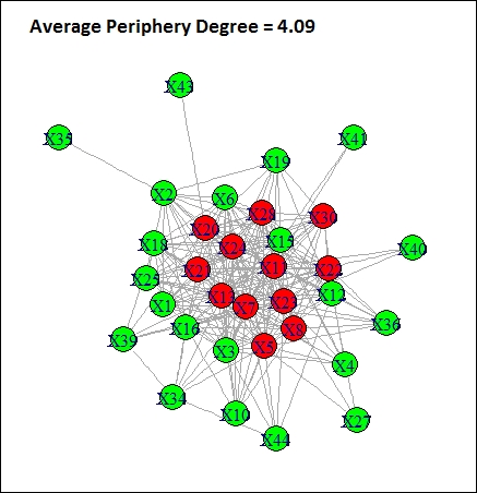
Figure 13.5: Core-periphery decomposition with the smallest periphery degree