This section explains the intra-day volume forecasting model proposed by Bialkowski, J., Darolles, S., and Le Fol, G. (2008).

They use CAC40 data to test their model, including the turnover of every stock in the index as of September 2004. Trades are aggregated into 20-minute time slots, resulting in 25 observations each day.

Turnover is decomposed into two additive components. The first one is the seasonal component (the U shape) that represents the expected level of turnover on an average day for each stock. Given that every day is a little different from the average, there is a second one, the dynamic component, which shows the expected deviation from the average on a specific day.

The decomposition is carried out using the factor model of Bai, J. (2003). The initial problem is as follows:

Here, the X (TxN)-sized matrix contains the initial data, F (Txr) is the factor matrix, Λ' (Nxr) is the matrix of factor loadings, and e (TxN) is the error term. K stands for the common term, T stands for the number of observations, N stands for the number of stocks, and r stands for the number of factors.

The dimension of the XX' matrix is (TxT). After determining its eigenvalues and eigenvectors, Eig contains the eigenvectors that are related to the r largest eigenvalues. The estimated factor matrix is then determined as:

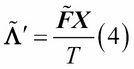
The transpose of the estimated loadings matrix is calculated as:

Finally, the estimated common component will be:

Given that the model is additive, the estimated dynamic component simply becomes:

Now that the estimated common and dynamic components are both obtained, the next step is to generate their forecasts. The authors assume that the seasonal (U shape) component is constant throughout the 20-day estimation period (but differs among stocks), so they forecast it according to:

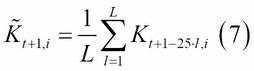
Knowing that 25 is the number of time slots (data points) each day, this means that for stock i, the forecast for the first time slot tomorrow will be the average of the first time slots during the last L days.

The forecast of the dynamic component is obtained in two different ways. One way is by fitting an AR(1) model, specified as follows:

Another way is by fitting a SETAR model, specified as:

Here, the indicator function is the following:

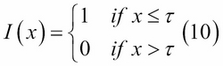
This means that if the previous observation does not exceed the threshold specified within the model, then the forecast is carried out by using one AR(1) model, and if it does, then the other AR(1) model is used.

After having forecasted both the seasonal and the dynamic components, the forecasted turnover will be the sum of the two:

Note that we have forecasted the dynamic component in two different ways; therefore, we will have two different forecast results depending on which one we add to the forecast of the seasonal component.