Building the required database could be one of the biggest challenges. Here, we do not only need dividend-adjusted price quotes but also financial statements data. Chapter 4, Big Data – Advanced Analytics described how to access some of the open data sources, but those rarely offer you all the required information in a package.

Another option might be to use professional financial data providers as a source. These platforms allow you to create tailor-made tables that can be exported to Microsoft Excel. For the sake of this chapter, we used a Bloomberg terminal. As a first step, we exported the data to Microsoft Excel.

Spreadsheets may be an excellent tool to build a database of data collected from different sources. No matter how you got your data ready on a spreadsheet, you need to notice that due to the changing output formats (xls, xlsx, xlsm, xlsb) and the advanced formatting features (for example, merging cells), this is not the best form to feed R with your data. Instead, you may be far better off with saving your data in a file in the comma-separated format or as CSVs. This can be easily read using the following commands:

d <- read.table("file_name", header = T, sep = ",")

Here, the = T header indicates that your database has a header row, and sep = "," indicates that your data is separated by commas. Note that some localized versions of Excel may use different separators, such as semicolons. In this case, use sep = ";". If your file is not located in your R working directory, you have to specify the whole path as part of file_name.

If you want to stick to your Excel file, the next method might work in most of the cases. Install the gdata package that extends the capabilities of R so that the software can read information form the xls or xlsx file:

install.packages("gdata")
library(gdata)

After that, you may read the Excel file as follows:

d <- read.xls("file_name", n)

Here, the second argument marked as n indicates the worksheet in the workbook from which you want to read.

To illustrate the process of building a fundamental trading strategy, we will use the NASDAQ Composite Index member firms. At the time of writing this chapter, 21,931 firms are included.

To create a solid base for our strategy, we should first clean our database. Extreme values may create a serious bias otherwise. For example, no one would be surprised if a firm with a P/E (Price/Earning per share) ratio of 150 a year ago showed a quick price increase during the last 12 months, but finding such a share now may be impossible, so our strategy might be worthless. The strategy should help us find what shares to invest in once the choice is not trivial (of course, you may also lose with high P/E shares), so we will only keep shares without extreme values. The following limitations were applied:

This way, only those firms remained that are not likely to be liquidated or go bankrupt, and they have shown performance that is clearly sustainable in the long run. After applying these filters, 7198 firms remained from all over the world.

The next step involves selecting the ratios we will potentially use when defining the strategy. Based on historical experience, we picked 15 ratios from the financial statements a year earlier, plus the name of the sectors the firms operate in and the total shareholder return for the last 12 months.

It may prove wise to check whether the remaining data is appropriate for our aims. A boxplot diagram would reveal whether, for example, most of our stocks show huge positive or negative return or whether there are heavy differences across industries due to which we would end up describing one given booming industry as not a good investment strategy. Luckily, here, we have no such issues: (Figure 1)

d <- read.csv2("data.csv", stringsAsFactors = F)
for (i in c(3:17,19)){d[,i] = as.numeric(d[,i])}
boxplot_data <- split( d$Total.Return.YTD..I., d$BICS.L1.Sect.Nm )
windows()
par(mar = c(10,4,4,4))
boxplot(boxplot_data, las = 2, col = "grey")

The following figure is the result of the preceding code:

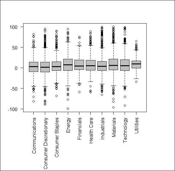
Figure 1

It could be also a good idea to check whether we should introduce new variables. One possible yet missing categorization could control for firm size, as many models assume higher required return for low capitalization stocks due to them being less liquid. To control this, we may apply a scatter diagram, the code and output for this is as follows:

model <- lm(" Total.Return.YTD..I. ~ Market.Cap.Y.1", data = d)
a <- model$coefficients[1]
b <- model$coefficients[2]
windows()
plot(d$Market.Cap.Y.1,d$Total.Return.YTD..I., xlim = c(0, 400000000000), xlab = "Market Cap Y-1", ylab = "Total Return YTD (I).")
abline(a,b, col = "red")

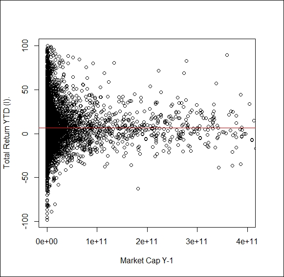
We cannot see a clear trend for capitalization and TRS. We may also try to fit a curve on the data and calculate R² for the goodness of the fit, but the figure does not support any strong connection. R square indicates the percentage of variance explained by your estimation, so any value above 0.8 is great, while values bellow 0.2 mean weak performance.