
Exchange options grant the holder the right to exchange one risky asset to another risky asset at maturity. It is easy to see that simple options are special forms of exchange options where one of the risky assets is a constant amount of money (the strike price).
The pricing formula of an exchange option was first derived by Margrabe, 1978. The model assumptions, the pricing principles, and the resultant formula of Margrabe are very similar to (more precisely, the generalization of) those of Black, Scholes, and Merton. Now we will show how to determine the value of an exchange option.
Let's denote the spot prices of the two risky assets at time t by S1t and S2t. We assume that these prices under the risk neutral probability measure (Q) follow geometric Brownian motion with drifts equal to the risk-free rate (r), shown as ![]() and
and ![]() .
.
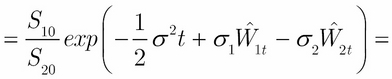
Here, W1 and W2 are standard Wiener processes under Q, with correlation ρ. You may observe that here, the assets have no yield (for example, stocks that pay no dividend). It is well known (and easy to see with Itô's lemma) that the solutions of the earlier mentioned stochastic differential equations are 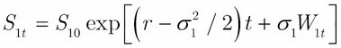 and
and 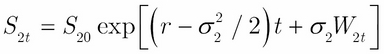 (1)
(1)
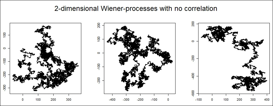
We assume that you are familiar with the basics of stochastic processes in one dimension. However, in the case of exchange options, we have a two-dimensional Wiener process, so it is useful to illustrate how this looks.
The 2D Wiener process is like a random walk in two dimensions and continuous time. We can easily generate such a process with a few lines of code when the coordinates are independent Wiener processes (not bothering ourselves with scaling the process because it looks the same).
D2_Wiener <- function() {
    dev.new(width = 10, height = 4)
    par(mfrow = c(1, 3), oma = c(0, 0, 2, 0))
    for(i in 1:3) {
        W1 <- cumsum(rnorm(100000))
        W2 <- cumsum(rnorm(100000))
        plot(W1,W2, type= "l", ylab = "", xlab = "")
    }
    mtext("2-dimensional Wiener-processes with no correlation",
        outer = TRUE, cex = 1.5, line = -1)
}
If we call this function, the output is something like this:
D2_Wiener()
Here, we can see the result in the following image:
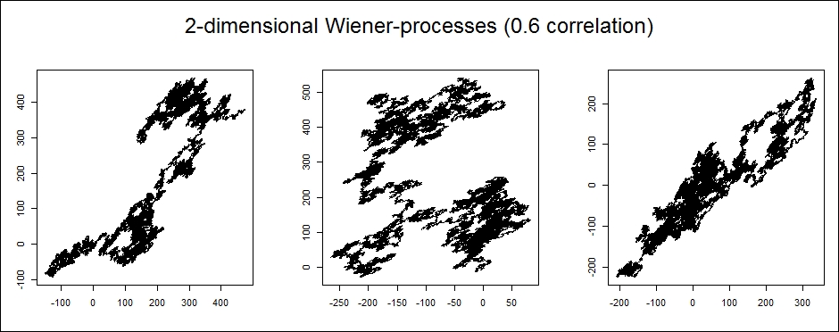
Correlation between the Wiener processes changes the picture dramatically. In the case of positive correlation, the two Wiener processes look like they are moving in the same direction; in the case of negative correlation, they look like they are moving in the opposite direction.
We can modify our function to get correlated Wiener processes. It is easy to see that the following code does the job:
Correlated_Wiener <- function(cor) {
    dev.new(width = 10, height = 4)
    par(mfrow = c(1, 3), oma = c(0, 0, 2, 0))
    for(i in 1:3) {
        W1 <- cumsum(rnorm(100000))
        W2 <- cumsum(rnorm(100000))
        W3 <- cor * W1 + sqrt(1 - cor^2) * W2
        plot(W1, W3, type= "l", ylab = "", xlab = "")
    }
    mtext(paste("2-dimensional Wiener-processes (",cor," correlation)",
          sep = ""), outer = TRUE, cex = 1.5, line = -1)
}
The result depends on the generated random numbers, but it is pretty much like this:
Correlated_Wiener(0.6)
Here, we can see the result in the following image:
In the previous example, we set the correlation coefficient to 0.6. Now, let's see what happens when it is -0.7:
Correlated_Wiener(-0.7)
Here, we can see the result in the following image:
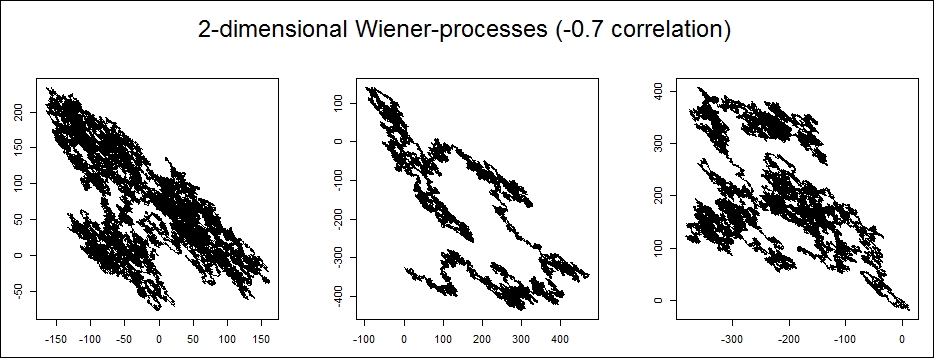
We can clearly see the difference between the processes with different correlations. Now, let's turn our attention back to exchange options.
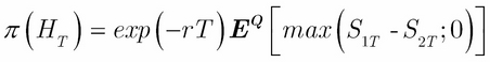
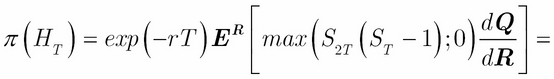
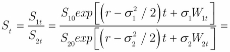
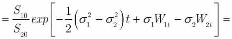
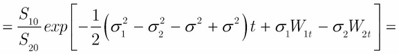
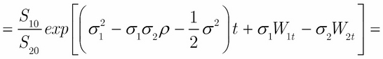
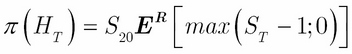
The payoff HT of the exchange option at maturity is defined by ![]() . According to the basic risk-neutral pricing principle, the value of this payoff (or equivalently, the price of the exchange option, denoted by π(HT)) is as follows:
. According to the basic risk-neutral pricing principle, the value of this payoff (or equivalently, the price of the exchange option, denoted by π(HT)) is as follows:
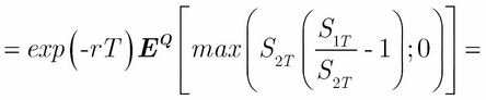
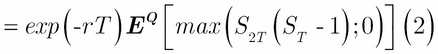
In Equation (2), St (without number 1 or 2 in the index) is defined as the S1t/S2t quotient. In other words, S is the price of S1 in terms of S2. If the two risky assets are two currencies, then S is an FX rate, and that is why we use this notation.
To calculate the earlier mentioned expected value, we need to introduce a new measure (R), defined by the following Radon-Nikodym derivative:
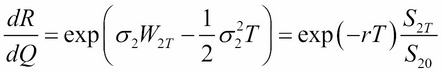
Here, the right-hand side of the earlier equation comes from Equation (1) for S2.
Then, the price of the exchange option will take the following form:
Now, we have to determine what kind of process S follows under R. From Girsanov's theorem, we know that ![]() and
and ![]() are Wiener processes under R, and their correlation is still ρ. Let's introduce the following two notations:
are Wiener processes under R, and their correlation is still ρ. Let's introduce the following two notations:
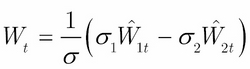
From Lévy's characterisation, we know that W is a Wiener process under R. Now we can determine the equation of S:
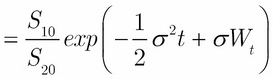
This means that S under R is a geometric Brownian motion with zero drift, that is ![]() .
.
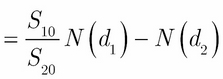
Now, if you remember, in Equation (3), we had the following equation for the price of the exchange option:
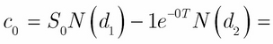
Using this relationship for S, the expected value at the right-hand side is the value of a simple call option with an underlying asset S, r is equal to 0, and X is equal to 1. Let's denote the price of this call option simply with c0. Then ![]() .
.
Here, c0 might be determined with the help of the basic Black-Scholes formula, substituting the parameters we just discussed:
Hence ![]()
where 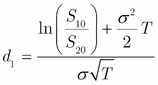 and
and 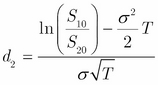
The previously mentioned formula for π(HT), which is the pricing formula for the exchange option, is called the Margrabe formula. Continuous dividend yields, if applicable, might be inserted into the formula as simply as in the case of the Black-Scholes formula. Without repeating the calculations, we give only the results for this case.
So, let's assume that the risky assets to be exchanged have positive continuous dividend yields denoted by δ1 and δ2 respectively. In this case, the processes of their prices under measure Q are as follows:
![]() and
and ![]()
In this case, the Margrabe formula will take the following form:
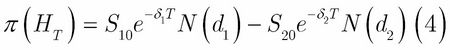
Here, 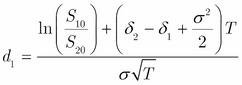 and
and 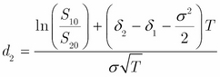 .
.
R has no built-in function for the Margrabe formula. However, it is much more difficult to understand the complex theory behind it than implement the result. Here, we present the Margrabe function only in a few lines, which calculates the price of the exchange option based on the parameters shown in the following code:
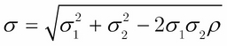
Margrabe <- function(S1, S2, sigma1, sigma2, Time, rho, delta1 = 0,
    delta2 = 0) {
    sigma <- sqrt(sigma1^2 + sigma2^2 - 2 * sigma1 * sigma2 * rho)
    d1 <- ( log(S1/S2) + ( delta2-delta1 + sigma^2/2 ) * Time ) /
        (sigma*sqrt(Time))
    d2 <- ( log(S1/S2) + ( delta2-delta1 - sigma^2/2 ) * Time ) /
        (sigma*sqrt(Time))
    M <- S1*exp(-delta1*Time)*pnorm(d1) - S2*exp(-delta2*Time)*pnorm(d2)
    return(M)
}
This is the core body of the function. If we are more demanding or want to develop a user-friendly application, we need to catch possible errors and exceptions. For example, we should include something like this:
if min(S1, S2) <= 0) stop("prices must be positive")
The execution should also be stopped when volatility is negative, but user-experience and related software design are beyond the scope of this book. We can use this function with valid parameters to see an example of how it works. Let's say we have two risky assets that pay no dividend, one with a price of 100 USD and 20 percent volatility, and the other with a price of 120 USD and 30 percent volatility, and the maturity is two years. At first, let the correlation be 15 percent.
We simply call the Margrabe function with the given parameters:
Margrabe(100, 120, .2, .3, 2, .15)
[1] 12.05247
The result is 12 USD. Now, let's see what happens if one of the assets is riskless, that is, its volatility is 0. Let's call the function with the following parameters:
Margrabe(100, 120, .2, 0, 2, 0, 0, 0.03)
[1] 6.566047
What does this mean? This product grants us the right to change the first risky asset, which is a stock that costs 100 USD with 20 percent volatility, to the second "risky" asset, which has a price of 120 USD, pays a 3 percent dividend, and has 0 volatility, (so it is a fixed cash amount) with 3 percent interest. Practically, in two years, it would be the right to buy the stock for 120 USD when the risk-free rate is 3 percent. Let's compare the price to the BS price of this call option:
BlackScholesOption("c", 100, 120, 2, 0.03, 0.03, .2)
Title:
 Black Scholes Option Valuation
Call:
 GBSOption(TypeFlag = "c", S = 100, X = 120, Time = 2, r = 0.03,
     b = 0.03, sigma = 0.2)
Parameters:
          Value:
 TypeFlag c
 S        100
 X        120
 Time     2
 r        0.03
 b        0.03
 sigma    0.2

Option Price:
 6.566058

Description:
 Tue Aug 05 11:29:57 2014
Yes, they are indeed the same. If we set the volatility of the first asset to 0, this practically means that we have a put option for the second asset.
Margrabe(100, 120, 0, 0.2, 2, 0, 0.03, 0)
[1] 3.247161
The result of the BS formula is as follows:
BlackScholesOption("p", 120, 100, 2, 0.03, 0.03, .2)

Title:
 Black Scholes Option Valuation

Call:
 GBSOption(TypeFlag = "p", S = 120, X = 100, Time = 2, r = 0.03,
     b = 0.03, sigma = 0.2)

Parameters:
          Value:
 TypeFlag p
 S        120
 X        100
 Time     2
 r        0.03
 b        0.03
 sigma    0.2

Option Price:
 3.247153

Description:
 Fri Aug 08 17:38:04 2014
In both cases, there is only a numeric error from the fifth digit.
We can also use the Margrabe formula to get the price of the currency option we discussed in the section Currency Options. We can check whether the BS formula provided the same price:
Margrabe(0.745, 0.7, 0.2, 0, 5, 0.15, 0.02, 0.03)
[1] 0.152222
The last thing we need to discuss is how correlation affects the price of the option. To illustrate this, we calculate the Margrabe price of the option for different values of correlation. This can be done with a few lines of code:
x <- seq(-1, 1, length = 1000)
y <- rep(0, 1000)
for (i in 1:1000)
    y[i] <- Margrabe(100, 120, .2, 0.3, 2, x[i])
plot(x, y, xlab = "correlation", ylab = "price",
    main = "Price of exchange option", type = "l", lwd = 3)
Here, we can see the result in the following image:
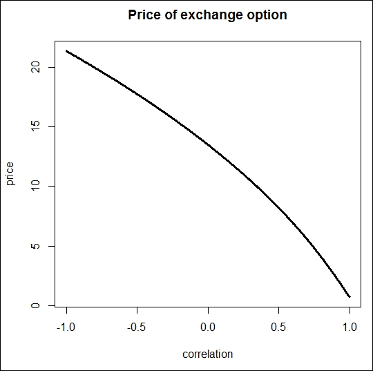
The result is not surprising. When correlation is high, we have the right to switch between identical stocks, which, clearly, is worth nothing. When the correlation is high on the negative side, we have better chances to make a good deal with the option if things go wrong (which means that if our asset decreases, the higher the negative correlation, the higher the chance that the price of the other asset increases and saves us from loss). In other words, in this case, the option is for insurance rather than speculation; we do not have to bear the risk from the price change of the other asset. This is why the option is more valuable when correlation is negative.