
Interest rate derivatives are financial derivative products whose payoff is dependent on the interest rates.
There is a wide range of such products; the basic types include interest rate swaps, forward rate agreements, callable and puttable bonds, bond options, caps and floors, and so on.
In this chapter, we will start with the Black model (also referred to as the Black-76 model), which is a generalized version of the Black-Scholes model, and is often used to price interest rate derivatives. Then, we will show how to apply the Black model to price an interest rate cap.
A shortcoming of the Black model is that it assumes lognormal distribution for some underlying asset (for example, bond price or interest rate), and it neglects how interest rate changes across time. Consequently, Black's formula cannot be used for all kinds of interest rate derivatives. Sometimes, it is necessary to model the term structure of interest rate models. There are plenty of interest rate models that try to capture the main features of this term structure. In the second part of this chapter, we discuss two basic and frequently used interest rate models, namely the Vasicek and the Cox-Ingersoll-Ross models. As in the previous chapter, we will assume that you are familiar with the Black-Scholes model and the basics of risk-neutral valuation.
We started this chapter by defining interest rate derivatives as assets with interest-rate-dependent cash flows. It is worth noting that the value of financial products is almost always dependent on some interest rates because of the need to discount the future cash flows. However, in the case of interest rate derivatives, not only the discounted value but the payoff itself depends on the interest rates. This is the main reason why interest rate derivatives are more complicated to price than stock or FX derivatives (Hull, 2009 discusses these difficulties in detail).
The Black model (Black, 1976) was developed to price options on futures contracts. Futures options grant the holder the right to enter into a futures contract at a predetermined futures price (strike price or exercise price, X) on a specified date (maturity, T). In this model, we keep the assumptions of the Black-Scholes model, except that the underlying is the futures price instead of the spot price. Hence, we assume that the futures price (F) follows a geometric Brownian motion:
It is easy to see that futures contracts might be handled as products with a continuous growth rate that is equal to the risk-free interest rate (r). Thus, it is not surprising that Black's formula for futures options is exactly the same as the Black-Scholes formula for currency options (discussed in the previous chapter), with q equal to r (as if the domestic and foreign interest rates were the same). So, Black's formula for a European futures call option is as follows:
Here, 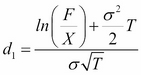 and
and 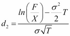 .
.
The price of a similar put option is as follows:
It is not a surprise that the GBSOption function (or the BlackScholesOption function) is useful for the Black model too. It is time to have a closer look at how it actually works.
When a function's name is typed in the R console without parenthesis, the function will not be called, but the source code is returned (except for byte-compiled code). This is not recommended for beginners, but it can be extremely useful for programmers with some experience because these details are usually not included in package documentation. Let's try it:
require(fOptions)
GBSOption
function (TypeFlag = c("c", "p"), S, X, Time, r, b, sigma, title = NULL,
    description = NULL)
{
    TypeFlag = TypeFlag[1]
    d1 = (log(S/X) + (b + sigma * sigma/2) * Time)/(sigma * sqrt(Time))
    d2 = d1 - sigma * sqrt(Time)
    if (TypeFlag == "c")
        result = S * exp((b - r) * Time) * CND(d1) - X * exp(-r *
            Time) * CND(d2)
    if (TypeFlag == "p")
        result = X * exp(-r * Time) * CND(-d2) - S * exp((b -
            r) * Time) * CND(-d1)
    param = list()
    param$TypeFlag = TypeFlag
    param$S = S
    param$X = X
    param$Time = Time
    param$r = r
    param$b = b
    param$sigma = sigma
    if (is.null(title))
        title = "Black Scholes Option Valuation"
    if (is.null(description))
        description = as.character(date())
    new("fOPTION", call = match.call(), parameters = param, price = result,
        title = title, description = description)
}
<environment: namespace:fOptions>
Do not worry if this is not totally clear; we are only interested in the computation of the price of the call option. First, d1 is calculated (we will check the formula in a minute). The BS formula has different forms (for stock options, currency options, and stock options with dividend), but the following equation always holds:
In the function, d2 is calculated based on this equation. The final result has the form ![]() , where a and b are dependent on the model but are always the discounted value of the price of the underlying and the strike price.
, where a and b are dependent on the model but are always the discounted value of the price of the underlying and the strike price.
Now, we can see the role of the b parameter in the calculation. As we mentioned in the previous chapter, this is how we can decide which model we want to use. If we carefully check the formulas, we can conclude that by setting b = r, we get the Black-Scholes stock option model; with b = r-q, we get Merton's stock option model with continuous dividend yield q (which is the same as the currency option model, as we saw in the previous chapter); and with b = 0, we get Black's futures option model.
Now, let's see an example of the Black model.
We need an option for an asset with 100 strike price in 5 years. The futures price is 120. Volatility of the asset is assumed to be 20%, and the risk-free rate is 5%. Now, simply call the BS option pricing formula with S = F and b = 0:
GBSOption("c", 120, 100, 5, 0.05, 0, 0.2)
We get the results in the usual form:
Title:
 Black Scholes Option Valuation
Call:
 GBSOption(TypeFlag = "c", S = 120, X = 100, Time = 5, r = 0.05,
     b = 0, sigma = 0.2)
Parameters:
          Value:
 TypeFlag c
 S        120
 X        100
 Time     5
 r        0.05
 b        0
 sigma    0.2

Option Price:
[1] 24.16356
The price of the option is about 24 USD, and we can also check from the output that b = 0, from which we must know that the Black model for futures options was used (or we made a serious mistake).
Although it was originally developed for commodity products, the Black model turned out to be a useful tool for pricing interest rate derivatives such as options on bonds or caps and floors. In the next section, we show how to use this model to price an interest rate cap.
Interest rate caps are interest rate derivatives where the holder receives positive payments throughout a number of time periods if the interest rate exceeds a certain level (the strike price, X). Analogously, the holder of an interest rate floor receives positive payments in each period if the interest rate is below the strike price. It is obvious that caps and floors are efficient products to hedge against interest rate volatility. In this section, we will discuss the pricing of a cap. Let's assume that the underlying rate is the LIBOR, L.
As we discussed in the previous chapter, the best way to understand derivatives is to determine their payoff structure. The payoff of a cap (with one unit of notional amount) at the end of the nth period is as follows:
Here, τ is the time interval between two payments. This single payment is called a caplet, and the cap is, of course, a portfolio of sequential caplets. When pricing a cap, all the caplets must be valued and then their prices have to be summed. Furthermore, the earlier mentioned payoff shows us that pricing the nth caplet is nothing but pricing a call option with the underlying asset of the Libor, strike price X, and maturity τn.
If we assume that the Libor rate at time n-1 (Ln-1) is a random variable that has lognormal distribution and the volatility is ![]() , then we can use Black's formula to price the caplet:
, then we can use Black's formula to price the caplet:
Here, 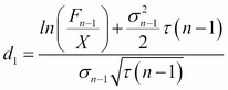 and
and  .
.
Here, Fn-1 is the forward Libor rate between τ(n-1) and τn, and r is the risk-free spot log return with maturity τn. Once we have the value of one single caplet, we can price all of them to get the price of the cap.
Let's see an example to understand this in depth. We have to pay USD LIBOR for 6 months to a business partner between May 2014 and November 2014. A caplet is an easy way to avoid the interest rate risk. Assume that we have a caplet on the LIBOR rate with 2.5% strike price (using the usual terminology).
This means that if the LIBOR rate is higher then 2.5%, we will receive the difference in cash. If, for example, the LIBOR rate turns out to be 3% in May, our payoff on one unit of notional amount is 0.5*max(3% -2.5%, 0).
Now, let's see how to price the caplet. There is nothing new in it; we can simply use the Black-Scholes formula. It is clear that we need to set S = Fn-1, Time = 0.5, and b = 0. Assuming that the LIBOR rate follows the geometric Brownian motion with 20% volatility, the forward rate between May 1st and November 1st is 2.2%, and the spot rate is 2%. In this case, the price of the caplet is as follows:
GBSOption("c", 0.022, 0.025, 0.5, 0.02, 0, 0.2)
Title:
 Black Scholes Option Valuation
Call:
 GBSOption(TypeFlag = "c", S = 0.022, X = 0.025, Time = 0.5, r = 0.02,
     b = 0, sigma = 0.2)
Parameters:
          Value:
 TypeFlag c
 S        0.022
 X        0.025
 Time     0.5
 r        0.02
 b        0
 sigma    0.2
Option Price:
 0.0003269133
The price of the option is 0.0003269133. We still need to multiply it with τ = 0.5, which makes it 0.0001634567. If we measure everything in million USD, this means that the price of the caplet is about 163 USD.
A cap is simply a sum of caplets, but we can combine them with different parameters if needed. Let's say we need a cap that pays if the LIBOR rate goes above 2.5% in the first 3 months, or if it is higher than 2% in the following 3 months. The forward LIBOR rate can also be different in the May and August period (let's say it is 2.1%), and in the August and November period (let's say it is 2.2%). We simply price both caplets one by one and add their prices:
GBSOption("c", 0.021, 0.025, 0.25, 0.02, 0, 0.2)
GBSOption("c", 0.022, 0.02, 0.25, 0.02, 0, 0.2)
We do not include all the outputs here, only the prices:
Option Price:
 3.743394e-05
Option Price:
 0.002179862
Now, we need to multiply both with τ = 0.25 and take the sum of their prices:
(3.743394e-05 + 0.002179862 ) * 0.25
0.000554324
The price of this cap with a notional amount of 1 million is about 554 USD.
Pricing a floor is very similar. First, we divide the asset's cash flows into single payments, called floorlets. Then, we determine the value of each floorlet with the help of the Black model; the only difference is that floorlets are not call but put options. Finally, we add up the prices of the floorlets to get the value of the floor.
Black's model is applicable when we can assume that the future value of the underlying asset has lognormal distribution. Another approach to value interest rate derivatives is by modeling the term structure of interest rates. Here, we continue by presenting two basic interest rate models and their main characteristics.