
In most of the cases in finance, valuation of financial assets is based on the discounted cash flow method; hence, the present value is calculated as the discounted value of the expected future cash flows. Therefore, in order to be able to value assets, we need to know the appropriate rate of return that reflects the time value of money and also the risk of the given asset. There are two main approaches to determine expected returns: the capital asset pricing model (CAPM) and the arbitrage pricing theory (APT). CAPM is an equilibrium model, while APT builds on the no-arbitrage principle; thus, these approaches have quite different starting points and inner logic. However, the final pricing formula we get can be quite similar, depending on the market factors we use. For the comparison of CAPM and APT, see Bodie-Kane-Marcus (2008). When we test any of these theoretical models on real-world data, we perform linear regressions. This chapter focuses on APT, since we have discussed CAPM in more detail in Daróczi et al. (2013).
This chapter is divided into two parts. In the first part, we introduce the theory of APT in general, and then we present a special three-factor model published in a seminal paper of Fama and French. In the second part, we show how to use R for data selection and how to estimate the pricing coefficients from real market data, and finally we re-examine the famous Fama-French model on a more recent sample.
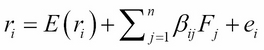
APT relies on the assumption that asset returns in the market are determined by macroeconomic and firm-specific factors, and asset returns are generated by the following linear factor model:
Equation 1
Here, E(ri) is the expected return of asset i, Fj stands for the unexpected change of the jth factor, and βij shows the ith security's sensitivity for that factor, while ei is the return caused by unexpected firm-specific events. So ![]() represents the random systemic effect, and ei represents the non-systemic (that is idiosyncratic) effect, which is not captured by the market factors. Being unexpected, both
represents the random systemic effect, and ei represents the non-systemic (that is idiosyncratic) effect, which is not captured by the market factors. Being unexpected, both ![]() and ei have a zero mean. In this model, factors are independent of each other and the firm-specific risk. Thus, asset returns are derived from two sources: the systemic risk of the factors that affect all assets in the market and the non-systematic risk that impacts only that special firm. A non-systemic risk can be diversified by holding more assets in the portfolio. In contrast, a systemic risk cannot be diversified, as it is caused by economy-wide sources of risks that affect the overall stock market (Brealey-Myers, 2005).
and ei have a zero mean. In this model, factors are independent of each other and the firm-specific risk. Thus, asset returns are derived from two sources: the systemic risk of the factors that affect all assets in the market and the non-systematic risk that impacts only that special firm. A non-systemic risk can be diversified by holding more assets in the portfolio. In contrast, a systemic risk cannot be diversified, as it is caused by economy-wide sources of risks that affect the overall stock market (Brealey-Myers, 2005).
As a consequence of the model, the realized return of an asset is the linear combination of multiple random factors (Wilmott, 2007).
Other important assumptions of APT are as follows:
- There are a finite number of investors on the market who optimize their portfolio for the next period. They are equally informed and have no market power.
- There is a riskless asset and an infinite number of risky assets traded continuously; thus, firm-specific risks can be totally eliminated by diversification. A portfolio that has zero firm-specific risks is called a well-diversified portfolio.
- Investors are rational in the sense that if an arbitrage opportunity occurs (financial assets are mispriced relative to each other), then investors immediately buy the underpriced security/securities and sell the overpriced one(s), and they will take an infinitely large position in order to earn as much riskless profit as possible. Consequently, any mispricing will disappear on the spot.
- Factor portfolios exist, and they are continuously tradable. A factor portfolio is a well-diversified portfolio that reacts only to one of the factors; specifically, it has a beta of 1 for that specified factor and a beta of 0 for all other factors.
From the preceding assumptions, it can be shown that any portfolio's risk premium equals the weighted sum of the factor portfolios' risk premium (Medvegyev-Száz, 2010). The following pricing formula can be derived in the case of a two-factor model:
Equation 2
Here, ri is the return of the ith asset, rf is the risk-free return, βi1 is the sensitivity of the ith stock's risk premium to the first systemic factor, and (r1-rf) is the risk premium of this factor. Similarly, βi2 is the sensitivity of the ith stock's risk premium to the second factor's excess return (r2-rf).
When we implement APT, we perform a linear regression in the following form:
Equation 3
Here, αi stands for a constant and εi is the asset's non-systemic, firm-specific risk. All other variables are the same as mentioned previously.
If there is only one factor in the model, and it is the return of the market portfolio, the pricing equation of the CAPM model and APT model will coincide:
Equation 4
In this case, the formula to be tested on real market data is as follows:
Equation 5
Here, ![]() is the return of a market portfolio represented by a market index (like the S&P 500). This is why we call Equation (5) the index model.
is the return of a market portfolio represented by a market index (like the S&P 500). This is why we call Equation (5) the index model.
The implementation of APT can be split into four steps: identifying the factors, estimating the factor coefficient, estimating the factor premiums, and pricing with APT (Bodie et al. 2008):
- Identifying the factors: As APT mentions nothing about the factors, they have to be identified empirically. These factors are usually macroeconomic factors, like stock market return, inflation, business cycle, and so on. The main problem in using macroeconomic factors is that factors are usually not independent of each other. The identification of the factors is often carried out by factor analysis. However, factors identified by factor analysis cannot necessarily be interpreted in an economically meaningful way.
- Estimating factor coefficients: In order to estimate the coefficients in a multivariate linear regression model, a general version of Equation (3) is used.
- Estimating the factor premiums: The estimation of the factor premiums is based on historical data, taking the average of the historical time-series data of the premiums of the factor portfolios.
- Pricing with APT: Equation (2) is used for calculating the expected return of any asset by substituting the appropriate variables into the equation.
Fama and French proposed a multifactor model in 1996, in which they used corporate indicators as factors instead of macroeconomic factors, since they found that these factors better describe the systemic risk of assets. Fama and French (1996) extended the index model by adding the firm size and the book-to-market ratio as return-generating factors to the market portfolio returns (Fama and French, 1996).
The firm size factor was constructed by taking the difference between the returns of small and large firms (rSMB). The name of the variable was SMB, which is derived from "small minus big". The book-to-market factor was calculated by taking the difference between firms' returns that have a high and low book-to-market ratio (rHML). The name of the variable was HML, which is derived from "high minus low".
Their model was the following:
Equation 6
Here, αi is a constant, which shows the abnormal rate of return, rf is the risk-free return, and βiHML is the ith asset's sensitivity to the book-to-market factor, while βiSMB is the ith asset's sensitivity to the factor of size, βiM is the sensitivity of the ith stock's risk premium to the market index factor, (rM-rf) is the risk premium of this factor, and ei is the asset's non-systemic, firm-specific risk with zero mean.