Most of the time, exotic options are traded in camouflage; they are embedded in structured bonds or certificates. The exotic behavior is translated into a much more user-friendly language that is easier to understand by an everyday investor. For example, a binary payout can be calculated into a coupon yield; the investor gets a higher coupon if the circumstances let the binary option give its payout. A structure that includes a knock-out option could be called an airbag certificate, since as far as a long KO option is not knocked-out, it gives some protection against market losses, similar to an airbag that protects the driver in case of a less serious accident.

Another example is a turbo certificate, which, most of the time, is just a securitized form of a knock-out option with a deep in-the-money strike and a KO close to the strike. Lookback options can be found in capital guarantee products with coupons linked to the extreme values of stock indices.

As a numerical example, let's take a look at a three-month maturity certificate of deposit (CD) that either pays a 3 percent coupon or 0 percent, conditionally on the FX market behavior. This capital-guaranteed product can be seen as a portfolio of a T-Bill and a binary option. If the 3-month T-bill can be purchased at 99.75 percent, then there is 0.25 cent on each dollar that can be spent on a binary option. The capital at maturity will be granted by the T-Bill part, while the binary option will be responsible for the contingent 3 percent coupon.

At this point, any binary option would do the trick; purchasing a DNT would work too, but there are way too many parameters. Banks must fine-tune all the parameters to make the whole construction attractive. In the risk-neutral world from the market makers' point of view, a lower trigger of L=0.9200 with a 3-month maturity is almost the same as L=0.9195, with a bit more than a 3-month maturity:

dnt1(0.9266, 1000000, 0.9600, 0.9200, 0.06, 90/365, 0.0025, -0.025)
[1] 50241.58
dnt1(0.9266, 1000000, 0.9600, 0.9195, 0.06, 94/365, 0.0025, -0.025)
[1] 50811.61

This is a very common feature among options, including knock-out events; some extra time can most of the time compensate for pushing the barrier a bit further from the spot. In the risk-neutral world, the S/L distance is always divided by a factor of , so there is a trade-off; we can make L lower, but in return, we should increase the maturity. In the real world, the expectations of end users are driven by their subjective or perceived probabilities. Provided that we are not planning to dynamically hedge our DNT, we would prefer L = 0.9195 and T = 94 days over L = 0.9200 and T = 90 days.

That is why L, U, and T should be set in a way that helps the product look attractive to end users. Also, if the exotic option is embedded into a structure, the structure itself should be easy to sell. At the end, most of the structures will be cut into smaller, retail-sized pieces, like 1000 USD notional. Of course, each slice of the cake will be the same, so for the bank, it can be seen as one huge product.

Coming back to setting L, U, and T, it is easy to see that the price of a DNT is strictly a monotone function of L, U, and T (and also a monotone for volatility). Under certain market conditions (S, r, b, and volatility), we set, say, L = 0.9195 and T = 94 days. Now, we can ask the following inverse pricing question: for what U will the price of the DNT be 33 percent of the payout?

This will be the implied upper barrier, implied in a sense that the price is already given. Here comes a strange answer: it is not certain that such an implied U exists! This is because if we start increasing the upper barrier, the DNT price will converge to the price of a No-Touch (NT) option. If this NT is worth less than 33 percent, no U will make our DNT worth 33 percent. We use the BinaryBarrierOption function from the fExoticOptions package to price the No-Touch option which is depicted in the following code:

dnt1(0.9266, 1000000, 1.0600, 0.9200, 0.06, 94/365, 0.0025, -0.025)
[1] 144702
a <- BinaryBarrierOption(9, 0.9266, 0, 0.9200, 1000000, 94/365, 0.0025, -0.025, 0.06, 1, 1, title = NULL, description = NULL)
(z <- a@price)
[1] 144705.3

In the risk-neutral world, if we push U 1000 pips higher, it will become almost completely irrelevant, so DNT behaves like an NT.

So, in this case, if we want the DNT to cost 33 percent, we should choose an L that is lower than 0.9195. Next, we set L = 0.9095 and find a U that makes the DNT worth 33 percent. At the end of this part, we will show a way to find an implied U by using the implied_U_DNT function which is shown in the following code. Now, suppose we use U = 0.9745 for other reasons.

dnt1(0.9266, 100, 0.9705, 0.9095, 0.06, 90/365, 0.0025, -0.025)
[1] 31.44338

This DNT costs only 31.44 percent of the payout, so there will still be some room for the bank to have some profit for all the hard work of structuring. Suppose the bank can sell a total of USD 100 million of this CD, then 3 months later, the bank has to pay to the clients either USD 100 million (0 percent per annum) or USD 100.75 million (approximately 3 percent per annum). This contingent promise can be hedged by purchasing T-Bills in 100 million USD notional and DNT options with 0.75 million USD payout. At the beginning, these instruments cost the bank 99.75%*100.000.000+31.44338%*750.000 = USD 99.985.825,35; thus, the bank makes a profit of 14,174.65 USD.

In other cases, the implied time to maturity could be an interesting question. Under certain market conditions (where S, r, b, and volatility are given) for a given (L,U) pair, what is the T that makes the DNT cost, say, 50 percent? Even for a very tight (L-U) interval, we can find a T small enough to make the DNT price go up to 50 percent; this is also true the other way round; even a very wide (L,U) pair will make a DNT worth only 50 percent if there is enough time. See implied_T_DNT at the end of this section.

Unlike L, U, or T, we cannot choose the volatility parameter deliberately; however, calculating the implied volatility could be useful to price other derivatives. This is a key pricing concept; risk-neutral pricing is based on comparison. If we know the price (and all other parameters) of a DNT, we can find out what volatility was used for pricing. See implied_vol_DNT at the end of this section.

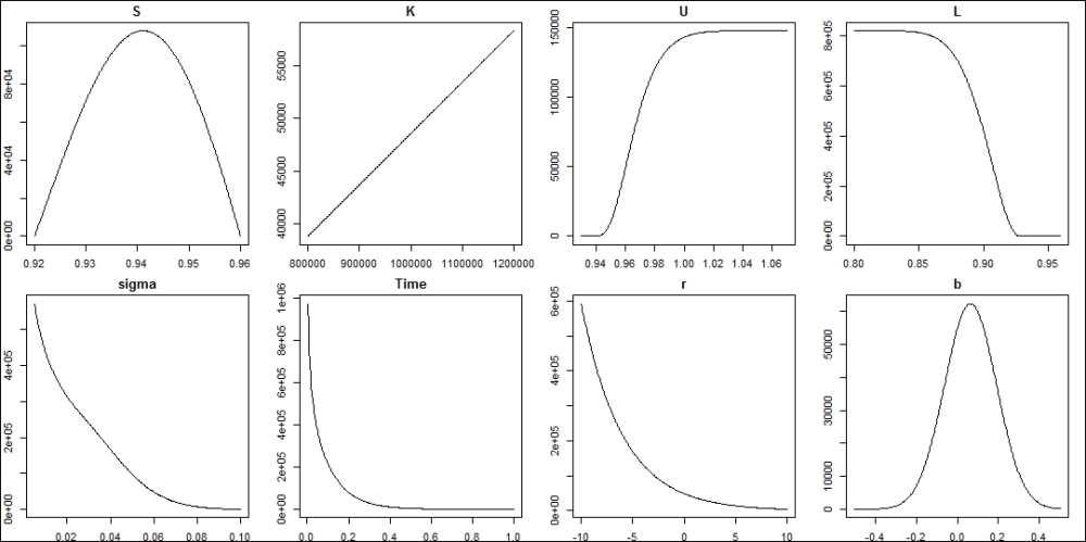
Next, we will show a lot of implied functions and finally draw the implied charts:

implied_DNT_image <- function(S = 0.9266, K = 1000000, U = 0.96,
  L = 0.92, sigma = 0.06, Time = 0.25, r = 0.0025, b = -0.0250) {
    S_ <- seq(L,U,length = 300)
    K_ <- seq(800000, 1200000, length = 300)
    U_ <- seq(L+0.01, L + .15, length = 300)
    L_ <- seq(0.8, U - 0.001, length = 300)
    sigma_ <- seq(0.005, 0.1, length = 300)
    T_ <- seq(1/365, 1, length = 300)
    r_ <- seq(-10, 10, length = 300)
    b_ <- seq(-0.5, 0.5, length = 300)

    p1 <- lapply(S_, dnt1, K = 1000000, U = 0.96, L = 0.92,
      sigma = 0.06, Time = 0.25, r = 0.0025, b = -0.0250)
    p2 <- lapply(K_, dnt1, S = 0.9266, U = 0.96, L = 0.92,
      sigma = 0.06, Time = 0.25, r = 0.0025, b = -0.0250)
    p3 <- lapply(U_, dnt1, S = 0.9266, K = 1000000, L = 0.92,
      sigma = 0.06, Time = 0.25, r = 0.0025, b = -0.0250)
    p4 <- lapply(L_, dnt1, S = 0.9266, K = 1000000, U = 0.96,
      sigma = 0.06, Time = 0.25, r = 0.0025, b = -0.0250)
    p5 <- lapply(sigma_, dnt1, S = 0.9266, K = 1000000, U = 0.96,
      L = 0.92, Time = 0.25, r = 0.0025, b = -0.0250)
    p6 <- lapply(T_, dnt1, S = 0.9266, K = 1000000, U = 0.96, L = 0.92, sigma = 0.06, r = 0.0025, b = -0.0250)
    p7 <- lapply(r_, dnt1, S = 0.9266, K = 1000000, U = 0.96, L = 0.92, sigma = 0.06, Time = 0.25,  b = -0.0250)
    p8 <- lapply(b_, dnt1, S = 0.9266, K = 1000000, U = 0.96, L = 0.92, sigma = 0.06, Time = 0.25, r = 0.0025)
    dev.new(width = 20, height = 10)

    par(mfrow = c(2, 4), mar = c(2, 2, 2, 2))
    plot(S_, p1, type = "l", xlab = "", ylab = "", main = "S")
    plot(K_, p2, type = "l", xlab = "", ylab = "", main = "K")
    plot(U_, p3, type = "l", xlab = "", ylab = "", main = "U")
    plot(L_, p4, type = "l", xlab = "", ylab = "", main = "L")
    plot(sigma_, p5, type = "l", xlab = "", ylab = "", main = "sigma")
    plot(T_, p6, type = "l", xlab = "", ylab = "", main = "Time")
    plot(r_, p7, type = "l", xlab = "", ylab = "", main = "r")
    plot(b_, p8, type = "l", xlab = "", ylab = "", main = "b")
}

implied_vol_DNT <- function(S = 0.9266, K = 1000000, U = 0.96, L = 0.92, Time = 0.25, r = 0.0025, b = -0.0250, price) {
    f <- function(sigma)
      dnt1(S, K, U, L, sigma, Time, r, b) - price
    uniroot(f, interval = c(0.001, 100))$root
}

implied_U_DNT <- function(S = 0.9266, K = 1000000, L = 0.92, sigma = 0.06, Time = 0.25, r = 0.0025, b = -0.0250, price = 4) {
    f <- function(U)
      dnt1(S, K, U, L, sigma, Time, r, b) - price
    uniroot(f, interval = c(L+0.01, L + 100))$root
}
implied_T_DNT <- function(S = 0.9266, K = 1000000, U = 0.96, L = 0.92, sigma = 0.06, r = 0.0025, b = -0.0250, price = 4){
    f <- function(Time)
        dnt1(S, K, U, L, sigma, Time, r, b) - price
    uniroot(f, interval = c(1/365, 100))$root
}
library(rootSolve)
implied_DNT_image()
print(implied_vol_DNT(price = 6))
print(implied_U_DNT(price = 4))
print(implied_T_DNT(price = 30))

The following is the output for the preceding code: