
In this chapter, we will deal with one of the biggest challenges of high-performance financial analytics and data management; that is, how to handle large datasets efficiently and flawlessly in R.
Our main objective is to give a practical introduction on how to access and manage large datasets in R. This chapter does not focus on any particular financial theorem, but it aims to give practical, hands-on examples to researchers and professionals on how to implement computationally - intensive analyses and models that leverage large datasets in the R environment.
In the first part of this chapter, we explained how to access data directly for multiple open sources. R offers various tools and options to load data into the R environment without any prior data-management requirements. This part of the chapter will guide you through practical examples on how to access data using the Quandl and qualtmod packages. The examples presented here will be a useful reference for the other chapters of this book. In the second part of this chapter, we will highlight the limitation of R to handle big data and show practical examples on how to load a large amount of data in R with the help of big memory and ff packages. We will also show how to perform essential statistical analyses, such as K-mean clustering and linear regression, using large datasets.
Extraction of financial time series or cross-sectional data from open sources is one of the challenges of any academic analysis. While several years ago, the accessibility of public data for financial analysis was very limited, in recent years, more and more open access databases are available, providing huge opportunities for quantitative analysts in any field.
In this section, we will present the Quandl and quantmod packages, two specific tools that can be used to seamlessly access and load financial data in the R environment. We will lead you through two examples to showcase how these tools can help financial analysts to integrate data directly from sources without any prior data management.
Quandl is an open source website for financial time series, indexing over millions of financial, economic, and social datasets from 500 sources. The Quandl package interacts directly with the Quandl API to offer data in a number of formats usable in R. Besides downloading data, users can also upload and edit their own data, as well as search in any of the data sources directly from R.upload and search for any data.
In the first simple example, we will show you how to retrieve and plot exchange rate time series with Quandl in an easy way. Before we can access any data from Quandl, we need to install and load the Quandl package using the following commands:
install.packages("Quandl")
library(Quandl)
library(xts)
We will download the currency exchange rates in EUR for USD, CHF, GBP, JPY, RUB, CAD, and AUD between January 01, 2005 and May 30, 2014. The following command specifies how to select a particular time series and period for the analysis:
currencies <- c( "USD", "CHF", "GBP", "JPY", "RUB", "CAD", "AUD")
currencies <- paste("CURRFX/EUR", currencies, sep = "")
currency_ts <- lapply(as.list(currencies), Quandl, start_date="2005-01-01",end_date="2013-06-07", type="xts")
As the next step, we will visualize the exchange rate evolution of four selected exchange rates, USD, GBP, CAD, and AUD, using the matplot() function:
Q <- cbind(
currency_ts[[1]]$Rate,currency_ts[[3]]$Rate,currency_ts[[6]]$Rate,currency_ts[[7]]$Rate)
matplot(Q, type = "l", xlab = "", ylab = "", main = "USD, GBP, CAD, AUD", xaxt = 'n', yaxt = 'n')
ticks = axTicksByTime(currency_ts[[1]])
abline(v = ticks,h = seq(min(Q), max(Q), length = 5), col = "grey", lty = 4)
axis(1, at = ticks, labels = names(ticks))
axis(2, at = seq(min(Q), max(Q), length = 5), labels = round(seq(min(Q), max(Q), length = 5), 1))
legend("topright", legend = c("USD/EUR", "GBP/EUR", "CAD/EUR", "AUD/EUR"), col = 1:4, pch = 19)
The following screenshot displays the output of the preceding code:
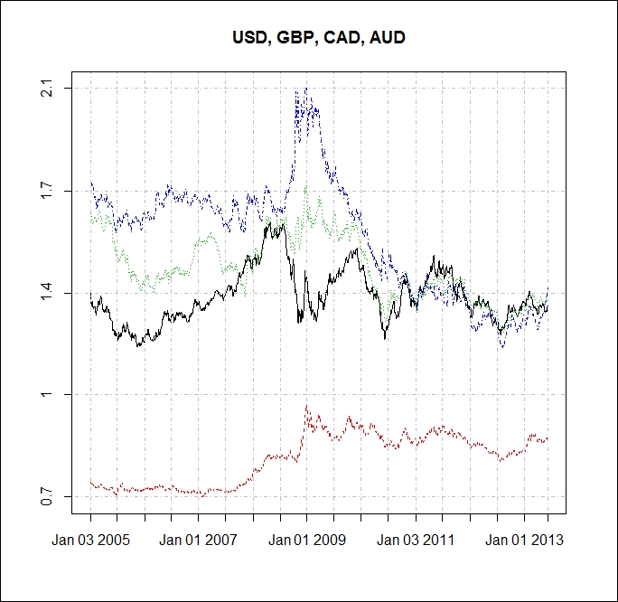
Figure 4.1: Exchange rate plot of USD, GBP, CAD, and AUD
In the second example, we will demonstrate the usage of the quantmod package to access, load, and investigate data from open sources. One of the huge advantages of the quantmod package is that it works with a variety of sources and accesses data directly for Yahoo! Finance, Google Finance, Federal Reserve Economic Data (FRED), or the Oanda website.
In this example, we will access the stock price information of BMW and analyze the performance of the car-manufacturing company since 2010:
library(quantmod)
From the Web, we will obtain the price data of BMW stock from Yahoo! Finance for the given time period. The quantmod package provides an easy-to-use function, getSymbols(), to download data from local or remote sources. As the first argument of the function, we need to define the character vector by specifying the name of the symbol loaded. The second one specifies the environment where the object is created:
bmw_stock<- new.env()
getSymbols("BMW.DE", env = bmw_stock, src = "yahoo", from = as.Date("2010-01-01"), to = as.Date("2013-12-31"))
As the next step, we need to load the BMW.DE variable from the bmw_stock environment to a vector. With the help of the head() function, we can also show the first six rows of the data:
BMW<-bmw_stock$BMW.DE
head(BMW)
           BMW.DE.Open BMW.DE.High BMW.DE.Low BMW.DE.Close BMW.DE.Volume
2010-01-04       31.82       32.46      31.82        32.05       1808100
2010-01-05       31.96       32.41      31.78        32.31       1564100
2010-01-06       32.45       33.04      32.36        32.81       2218600
2010-01-07       32.65       33.20      32.38        33.10       2026100
2010-01-08       33.33       33.43      32.51        32.65       1925800
2010-01-11       32.99       33.05      32.11        32.17       2157800
           BMW.DE.Adjusted
2010-01-04           29.91
2010-01-05           30.16
2010-01-06           30.62
2010-01-07           30.89
2010-01-08           30.48
2010-01-11           30.02
The quantmod package is also equipped with a finance charting ability. The chartSeries() function allows us to not only visualize but also interact with the charts. With its expanded functionality, we can also add a wide range of technical and trading indicators to a basic chart; this is a very useful functionality for technical analysis.
In our example, we will add the Bollinger Bands using the addBBands() command and the MACD trend-following momentum indicator using the addMACD() command to get more insights on the stock price evolution:
chartSeries(BMW,multi.col=TRUE,theme="white")
addMACD()
addBBands()
The following screenshot displays the output of the preceding code:
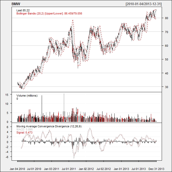
Figure 4.2: BMW stock price evolution with technical indicators
Finally, we will calculate the daily log return of the BMW stock for the given period. We would also like to investigate whether the returns have normal distribution. The following figure shows the daily log returns of the BMW stock in the form of a normal Q-Q plot:
BMW_return <-
log(BMW$BMW.DE.Close/BMW$BMW.DE.Open)
qqnorm(BMW_return, main = "Normal Q-Q Plot of BMW daily log return",
 xlab = "Theoretical Quantiles",
        ylab = "Sample Quantiles", plot.it = TRUE, datax = FALSE
 )
qqline(BMW_return, col="red")
The following screenshot displays the output of the preceding code. It shows the daily log returns of the BMW stock in the form of a normal Q-Q plot:
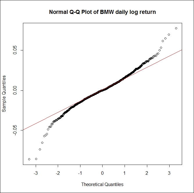
Figure 4.3: Q-Q Plot of the daily return of BMW