The value of a forward or futures contract depends on the spot price of the underlying asset, the time to maturity, the risk-free rate, and the strike price; in the case of plain vanilla options, the volatility of the underlying asset also has an effect on the option price. This statement holds only if the underlying asset provides no cash flow (no income and no cost) till the maturity of the derivative transaction; otherwise, this (both incoming and outgoing) cash flow also has an effect on the price. For the purpose of simplicity, here we will discuss derivatives pricing under the assumption of no cash flow (non-dividend-paying stocks), although an extension of the model to other underlying assets (like currencies and commodities) needs some modifications in the formulas, but it has no impact on the basic logic. As the strike price is stable during maturity, only changes to the other four factors can cause a change in the value of the derivative. The sensitivity of the derivative towards the mentioned variables is shown by the Greeks, the first partial derivatives according to the given variable, as presented in detail in Daróczi et al. (2013) Chapter 6, Derivatives Pricing.

The Black-Scholes-Merton model assumes that both the risk-free interest rate and the volatility of the underlying are constant, so as the change of time is deterministic, the only stochastic variable that affects the value of the derivative is the spot price of the underlying asset. The risk that is derived from the fluctuation of the spot price can be eliminated by holding the exact delta amount, which is the sensitivity of the derivative's price to the spot price (see Equation 1) of the underlying asset:

Equation 1

Whether delta is stable or changes over time depends on the derivative, and leads to different (static or dynamic) hedging strategies (Hull, 2009) presented in the following section.

Hedging of a forward agreement is straightforward as it is a binding obligation for both parties. Being in a long-forward position, we are sure that we will buy at maturity, while a short position means a sale of the underlying asset with certainty. So we can perfectly hedge our forward position by selling (long forward) or buying (short forward) the underlying at the amount of the derivative. We can check the delta of the forward by differentiating the value of the long-forward position:

Equation 2

Here, LF stands for the long forward, S denotes the spot price, and K is the strike price, which is the agreed forward price. The present value is denoted by PV.

So delta equals one, and it is independent of the actual market circumstances.

However, the value of a futures contract is the difference between the actual futures price (F) and the strike (S), because of the daily settlement of the position; hence, its delta is F/S and it changes with time. Consequently, a slight rebalancing of the position is needed, but in the absence of stochastic interest rates, the process of delta can be foreseen (Hull, 2009).

In the case of options, the delivery of the underlying is uncertain. It depends on the decision of the party in a long position; this is the party that bought the option. Not surprisingly, the hedging of a contingent claim cannot be achieved by a static buy-and-hold strategy presented in the previous point. In the framework of the binomial model, an option position is always hedged for the next Δt period, while in the Black-Scholes-Merton model, Δt converges to zero; thus, the hedging position is to be rebalanced in every instant. However, in the real world, practice assets can only be traded at discrete points of time, so the hedging portfolio is adjusted also at discrete time points. Let's look at the consequences of this in the example of a plain vanilla ATM (at-the-money) call option written on a non-dividend paying stock.

R contains a package, OptHedge, for the estimation of the value of an option and hedging strategy of call and put options on a grid at discrete time intervals; however, our aim is to illustrate the effect of the length of the trading periods. Therefore, we will use our own functions for the calculations.

First, we install the package to be used:

install.packages("fOptions")
library(fOptions)

Then, we can check the BS price of the call by using the already known code on a chosen parameter set:

GBSOption(TypeFlag = "c", S = 100, X = 100, Time = 1/2, r = 0.05, b = 0.05, sigma = 0.3)

We receive the given parameters and the price of the call option according to the Black-Scholes formula:

Parameters:
          Value:
 TypeFlag c     
 S        100   
 X        100   
 Time     0.5   
 r        0.05  
 b        0.05  
 sigma    0.3   
Option Price:
 9.63487 

Based on the BS model, the price of the call is 9.63487.

In practice, usually, the prices of the options are quoted in the standardized markets, and the implied volatility can be inferred from the Black-Scholes formula. A trader who expects lower volatility in the future than the implied volatility can make a profit by selling the option and simultaneously delta hedging it. In the following scenario, we present delta hedging of the short position in the preceding option on a stock following a geometric Brownian motion (GBM). We assume that all assumptions of the BSM model, except for the continuous-time trading, hold. In order to hedge the short option, we have to have delta amount of the stock, and as delta changes, we have to rebalance our portfolio regularly, in the following case, weekly, which makes it 26 times during the lifetime of the option. The frequency of the rebalancing should adjust to the liquidity and volatility of the underlying asset.

Let's look at a possible future path of the stock price and the development of the delta. The price_simulation function generates the price process with the given parameters: initial stock price (S₀), drift (mu), and volatility (sigma) of the GBM process and the remaining parameters of the call option (K, Time) and the chosen rebalancing period (Δt). After simulating the spot price process, the function calculates the delta and the price of the option for every interim date, and also plots them. By using the set.seed function, we can create reproducible simulations:

set.seed(2014)
library(fOptions)
Price_simulation <- function(S0, mu, sigma, rf, K, Time,  dt, plots = FALSE) {
  t <- seq(0, Time, by = dt)
  N <- length(t)
  W <- c(0,cumsum(rnorm(N-1)))
  S <- S0*exp((mu-sigma^2/2)*t + sigma*sqrt(dt)*W)
  delta <- rep(0, N-1)
  call_ <- rep(0, N-1)
  for(i in 1:(N-1) ){
    delta[i] <- GBSGreeks("Delta", "c", S[i], K, Time-t[i], rf, rf, sigma)
    call_[i] <- GBSOption("c", S[i], K, Time-t[i], rf, rf, sigma)@price}
  if(plots){
    dev.new(width=30, height=10)
    par(mfrow = c(1,3))
    plot(t, S, type = "l", main = "Price of underlying")
    plot(t[-length(t)], delta, type = "l", main = "Delta", xlab = "t")
    plot(t[-length(t)], call_ , type = "l", main = "Price of option", xlab = "t")
  }
}

We then set the parameters of our function:

Price_simulation(100, 0.2, 0.3, 0.05, 100, 0.5, 1/250, plots = TRUE)

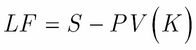
We will get a potential path of the stock price, the actual delta, and the corresponding option price:

We can see a possible future scenario, according to which the spot price rises and quickly arrives at an in-the-money level, so the option is exercised at maturity. The delta of the call follows the stock price's fluctuations and converges to one. The probability of exercising the call option increases if the spot price moves up, and in order to replicate the call, we have to buy some more stock, while the falling stock price leads to a lower delta, indicating a sale. All in all, we buy if the stock is expensive, and sell if the price is low. The price of the option derives from this cost of the hedging. The shorter the rebalancing period, the less the price movement that we have to follow.

The cost of hedging is defined as the present value of the cumulative net costs of buying and selling the stock (see Hull, 2009) needed to hedge the position. The total cost will have two parts, the amount paid to buy shares and the interest of financing the position. Following the BSM model, we use the risk-free interest rate for compounding. We will see that the cost of hedging depends on the future price movements, and by simulating several stock price paths, we can draw the cost distribution. Higher stock price volatility causes higher volatility of the cost of hedging.

The Cost_simulation function calculates the cost of hedging for the written call:

cost_simulation = function(S0, mu, sigma, rf, K, Time,  dt){
t <- seq(0, Time, by = dt)
N <- length(t)
W <- c(0,cumsum(rnorm(N-1)))
S <- S0*exp((mu-sigma^2/2)*t + sigma*sqrt(dt)*W)
delta <- rep(0, N-1)
call_ <- rep(0, N-1)
for(i in 1:(N-1) ){
delta[i] <- GBSGreeks("Delta", "c", S[i], K, Time-t[i], rf, rf, sigma)
call_[i] <- GBSOption("c", S[i], K, Time-t[i], rf, rf, sigma)@price
}

In the following command, share_cost represents the cost of buying the underlying asset to maintain the hedge position, and interest_cost is the cost of financing the position:

share_cost <- rep(0,N-1)
interest_cost <- rep(0,N-1)
total_cost <- rep(0, N-1)
share_cost[1] <- S[1]*delta[1]
interest_cost[1] <- (exp(rf*dt)-1) * share_cost[1]
total_cost[1] <- share_cost[1] + interest_cost[1]
for(i in 2:(N-1)){
    share_cost[i] <- ( delta[i] - delta[i-1] ) * S[i]
    interest_cost[i] <- ( total_cost[i-1] + share_cost[i] ) * (exp(rf*dt)-1)
    total_cost[i] <- total_cost[i-1] + interest_cost[i] + share_cost[i]
             }
c = max( S[N] - K , 0)
cost = c - delta[N-1]*S[N] + total_cost[N-1]
return(cost*exp(-Time*rf))
}

We can use the preceding defined function to generate different future price processes, based on which the cost of hedging can be calculated. Vector A collects several possible hedging costs and draws their histogram as a probability distribution. Next, we present hedging strategies, which rebalance weekly (A) and daily (B):

call_price = GBSOption("c", 100, 100, 0.5, 0.05, 0.05, 0.3)@price
A = rep(0, 1000)
for (i in 1:1000){A[i] = cost_simulation(100, .20, .30,.05, 100, 0.5, 1/52)}
B = rep(0, 1000)
for (i in 1:1000){B[i] = cost_simulation(100, .20, .30,.05, 100, 0.5, 1/250)}
dev.new(width=20, height=10)
par(mfrow=c(1,2))
hist(A, freq = F, main = paste("E = ",round(mean(A), 4) ,"  sd = ",round(sd(A), 4)), xlim = c(6,14), ylim = c(0,0.7))
curve(dnorm(x, mean=mean(A), sd=sd(A)), col="darkblue", lwd=2, add=TRUE, yaxt="n")
hist(B, freq = F, main = paste("E = ",round(mean(B), 4) ,"  sd = ",round(sd(B), 4)), xlim = c(6,14), ylim = c(0,0.7))
curve(dnorm(x, mean=mean(B), sd=sd(B)), col="darkblue", lwd=2, add=TRUE, yaxt="n")

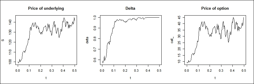
The output is the histogram of the generated cost outcomes:

The histogram on the left side shows the cost distribution of the weekly strategy, while the histogram on the right side belongs to the daily rebalancing strategy.

As we can see, the standard deviation of the cost of hedging can be reduced by shortening Δt, which indicates more frequent rebalancing of the portfolio. It is worth noticing that it is not only the volatility of the hedging cost that decreases with the shorter period, but the expected value is also lower, approaching the BS price.

We can further investigate the effect of the rebalancing period by making a slight modification to the cost simulation function by which the same future paths will be selected. In this way, we can compare strategies with a different rebalancing period.

The performance measure of delta hedging is defined by Hull (2009) as the ratio of the standard deviation of the cost of writing the option and hedging it to the theoretical price of the option.

The Cost_simulation function needs to be modified so that we can calculate several rebalancing periods together:

library(fOptions)
cost_simulation = function(S0, mu, sigma, rf, K, Time, dt, periods){
t <- seq(0, Time, by = dt)
N <- length(t)
W = c(0,cumsum(rnorm(N-1)))
S <- S0*exp((mu-sigma^2/2)*t + sigma*sqrt(dt)*W)
SN = S[N]
delta <- rep(0, N-1)
call_ <- rep(0, N-1)
for(i in 1:(N-1) ){
delta[i] <- GBSGreeks("Delta", "c", S[i], K, Time-t[i], rf, rf, sigma)
call_[i] <- GBSOption("c", S[i], K, Time-t[i], rf, rf, sigma)@price
}
S = S[seq(1, N-1, by = periods)]
delta = delta[seq(1, N-1, by = periods)]
m = length(S)
share_cost <- rep(0,m)
interest_cost <- rep(0,m)
total_cost <- rep(0, m)
share_cost[1] <- S[1]*delta[1]
interest_cost[1] <- (exp(rf*dt*periods)-1) * share_cost[1]
total_cost[1] <- share_cost[1] + interest_cost[1]
for(i in 2:(m)){
    share_cost[i] <- ( delta[i] - delta[i-1] ) * S[i]
    interest_cost[i] <- ( total_cost[i-1] + share_cost[i] ) * (exp(rf*dt*periods)-1)
    total_cost[i] <- total_cost[i-1] + interest_cost[i] + share_cost[i]
             }
c = max( SN - K , 0)
cost = c - delta[m]*SN + total_cost[m]                         
return(cost*exp(-Time*rf))
}

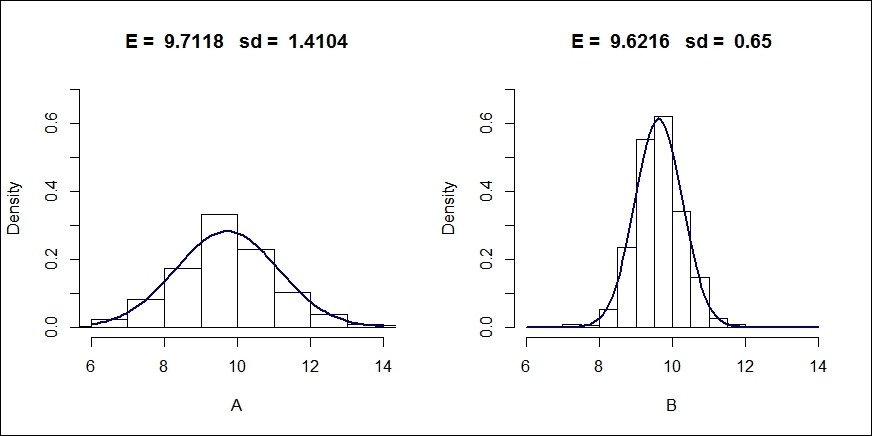
In the following command, the modified cost_simulation function is used for different rebalancing periods, and a table is generated that contains the expected value (E) with the lower and upper bound of the confidence level, the volatility of the cost of hedging (v), and the performance measure (ratio) ordered to the six rebalancing periods (0.5, 1, and 2 days, and 1, 2, and 4 weeks). We also receive two plots, the histograms of each strategy, and a chart that contains the normal curves fitted to the distributions:

dev.new(width=30,height=20)
par(mfrow = c(2,3))
i = 0
per = c(2,4,8,20,40,80)
call_price = GBSOption("c", 100, 100, 0.5, 0.05, 0.05, 0.3)@price
results = matrix(0, 6, 5)
rownames(results) = c("1/2 days", "1 day", "2 days", "1 week", "2 weeks", "4 weeks")
colnames(results) = c("E", "lower", "upper", "v", "ratio")
for (j in per){
  i = i+1
  A = rep(0, 1000)
  set.seed(10125987)
  for (h in 1:1000){A[h] = cost_simulation(100, .20, .30,.05, 100, 0.5, 1/1000,j)}
  E = mean(A)
  v = sd(A)
  results[i, 1] = E
  results[i, 2] = E-1.96*v/sqrt(1000)
  results[i, 3] = E+1.96*v/sqrt(1000)
  results[i, 4] = v
  results[i, 5] = v/call_price
  hist(A, freq = F, main = "", xlab = "", xlim = c(4,16), ylim = c(0,0.8))
  title(main = rownames(results)[i], sub = paste("E = ",round(E, 4) ,"  sd = ",round(v, 4)))
  curve(dnorm(x, mean=mean(A), sd=sd(A)), col="darkblue", lwd=2, add=TRUE, yaxt="n")
}
print(results)
dev.new()
curve(dnorm(x,results[1,1], results[1,4]), 6,14, ylab = "", xlab = "cost")
for (l in 2:6) curve(dnorm(x, results[l,1], results[l,4]), add = TRUE, xlim = c(4,16), ylim = c(0,0.8), lty=l)
legend(legend=rownames(results), "topright", lty = 1:6)

In our simulation model, the output is as follows:

                E    lower     upper         v    ratio
1/2 days 9.645018 9.616637  9.673399 0.4579025 0.047526
1 day    9.638224 9.600381  9.676068 0.6105640 0,06337
2 days   9.610501 9.558314  9.662687 0.8419825 0,087389
1 week   9.647767 9.563375  9.732160 1.3616010 0,14132
2 weeks  9.764237 9.647037  9.881436 1.8909048 0,196256
4 weeks  9.919697 9.748393 10.091001 2.7638287 0,286857

The standard deviation of the cost of hedging becomes smaller as we rebalance the hedge position more often. The difference in the expected value is also significant at 95 percent significance level between the weekly and the monthly the rebalancing. Among the shorter periods, we did not find significant differences in the expected value:

The charts shown in the preceding image are similar to the previous analysis (with weekly and daily rebalancing), but here, we have more rebalancing periods. The effect of rebalancing frequency is presented by the distribution of the cost of hedging.

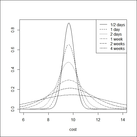
We can compare the cost distributions of the given rebalancing periods on a single chart, as illustrated in the preceding section.

The time consumption can be reduced by decreasing the number of simulations.