
Traditional liquidity risk measurement tools are the so-called static and dynamic liquidity gap tables. A liquidity gap table gives a cash-flow view of the balance sheet, and organizes the balance sheet items according to their contractual cash-inflows and cash-outflows into maturity buckets. The net cash-flow gap in each bucket shows the bank structural liquidity position. The static view assumes a rundown balance sheet while the dynamic liquidity table also takes into account the cash-flows from rollovers and new businesses. For the sake of simplicity, we demonstrate here only the static view of the liquidity positions.
Starting with the preparation of daily cash-flow positions. Sometimes, we need to know what the forecasted liquidity position is on a given date. It is easy to aggregate the cashflow.table by date.
head(aggregate(. ~ date, FUN = sum, data = subset(cashflow.table,select = -c(id, account))))
        date            cf    interest    capital remaining
1 2014-10-01   930.0387500   0.0387500   930.0000      0.00
2 2014-10-14     0.6246667   0.6246667     0.0000   3748.00
3 2014-10-15  2604.2058990 127.5986646  2476.6072  13411.39
4 2014-10-28   390.7256834 124.6891519   266.0365  23444.96
5 2014-10-30 -3954.2638670  52.6149502 -4006.8788 -33058.12
6 2014-10-31    -0.1470690  -0.1470690     0.0000  -2322.00
Secondly, let's prepare a liquidity gap table and create a chart. We can also use a predefined function (lq.table) and check the resulting table.
lq <- lq.table(cashflow.table, now = NOW)
round(lq[,1:5],2)
               1M    2-3M     3-6M    6-12M     1-2Y
afs_1        2.48 3068.51 14939.42     0.00     0.00
cb_1       930.04    0.00     0.00     0.00     0.00
cl_1      3111.11    0.00   649.51  2219.41  2828.59
cor_sd_1  -217.75 -217.73  -653.09 -1305.69 -2609.42
cor_td_1    -1.90 -439.66 -6566.03     0.00     0.00
is_1        -8.69  -17.48 -2405.31  -319.80  -589.04
mmp_1        0.16 2400.25     0.00     0.00     0.00
mmt_1       -0.12   -0.54    -0.80 -1201.94     0.00
oth_a_1      0.00    0.00     0.00     0.00     0.00
oth_l_1      0.00    0.00     0.00     0.00     0.00
rep_1     -500.05    0.00     0.00     0.00     0.00
ret_sd_1  -186.08 -186.06  -558.04 -1115.47 -2228.46
ret_td_1 -4038.96   -5.34 -5358.13 -3382.91     0.00
rm_1       414.40  808.27  1243.86  2093.42  4970.14
ro_1       466.67  462.50  1362.50  2612.50   420.83
total      -28.69 5872.72  2653.89  -400.48  2792.63
To plot the liquidity gap figure, we can use the barplot function, which is as follows:
plot.new()
par.backup <- par()
par(oma = c(1, 1, 1, 6), new = TRUE)
barplot(nii, density=5*(1:(NROW(nii)-1)), xlab="Maturity", cex.names=0.8, ylab = "EUR", cex.axis = 0.8, args.legend = list(x = "right"))
title(main = "Net interest income table", cex = 0.8, sub = paste("Actual date: ",as.character(as.Date(NOW))) )
par(fig = c(0, 1, 0, 1), oma = c(0, 0, 0, 0),mar = c(0, 0, 0, 0), new = TRUE)
plot(0, 0, type = "n", bty = "n", xaxt = "n", yaxt = "n")
legend("right", legend = row.names(nii[1:(NROW(nii)-1),]), density = 5*(1:(NROW(nii)-1)), bty = "n", cex = 1)
par(par.backup)
The output of the barplot function is as follows:
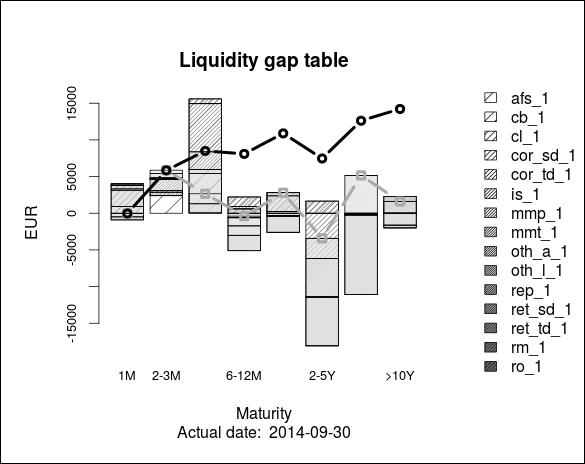
The bars on the plot show the liquidity gap in each time bucket. The dashed line with squares represents the net liquidity position (financial need), while the solid black line shows the cumulative liquidity gap.