Haug (2007a) comprehensively covers the collection of pricing formulas for around 100 exotic derivatives. The fOptions and fExoticOptions packages are based on this book. Wilmott (2006), Taleb (1997), and DeRosa (2011) describe a lot of practical issues about them.

The first impression could be that there are way too many exotic options. There are many ways of classification. Market makers talk about different generations of exotics, such as first generation, second generation, and so on. Their approach is from a hedging point of view. We will use a slightly different angle, the end-user approach, and classify the options based on their main exotic feature.

Asian type exotics are about the average. It could be an average rate or an average strike, and it could also be an arithmetic or geometric average. These options are path dependent; that is, their value at expiry is not purely a function of the underlying price at expiry but the total path. Asian options are cheaper than the vanillas since the volatility of the average price is lower than the volatility of the price itself:

library(fOptions)
library(fExoticOptions)
a <- GBSOption("c", 100, 100, 1, 0.02, -0.02, 0.3, title = NULL,
    description = NULL)(z <- a@price)
[1] 10.62678
a <- GeometricAverageRateOption("c", 100, 100, 1, 0.02, -0.02, 0.3,
    title = NULL, description = NULL)(z <- a@price)[1] 5.889822

Barrier type exotics are also path-dependent options. There could be one or two barriers. Each barrier could be either knock-in (KI) or knock-out (KO). During the lifetime of the option, the price of the underlying is monitored, and if it is traded at or over the barrier, there will be a knock event. Options with KI barriers become exercisable if the knock event occurs. Options with KO barriers start their life as exercisable options, however, they become non-exercisable if the knock event occurs. If there are two barriers, both of them could be the same type: double-knock-out (DKO) and double-knock-in (DKI), or it could be a knock-in-knock-out (KIKO) type.

If all other parameters are set to be the same, then the following equation holds:

KI + KO = vanilla.

This is because in this case, KI and KO options are mutually exclusive, but one of them will be exercisable for sure. The first parameters cuo and cui are flags for call-up-and-out and call-up-and-in. Next, we check for the following condition:

vanilla - KO - KI = 0.

The following code illustrates the preceding condition:

library(fExoticOptions)
a <- StandardBarrierOption("cuo", 100, 90, 130, 0, 1, 0.02, -0.02, 0.30,
    title = NULL, description = NULL)
x <- a@price
b <- StandardBarrierOption("cui", 100, 90, 130, 0, 1, 0.02, -0.02, 0.30, 
    title = NULL, description = NULL)
y <- b@price
c <- GBSOption("c", 100, 90, 1, 0.02, -0.02, 0.3, title = NULL, 
    description = NULL)
z <- c@price

v <- z - x - y
v
[1] 0

Based on the same logic of DKO + DKI = vanilla, we can even state that KO - DKO = KIKO. So, the KIKO options start as non-exercisable, and as long as both the short DKO and the long KO are alive, they neutralize each other. Should the short DKO die and the long KO survive, then it is a KI event for the KIKO option. However, the KIKO can still die even after being knocked-in. Naturally, the KIKO + DKO = KO approach leads to the same conclusion.

Also, there are some important convergence features among barrier options. Based on the KO + KI= vanilla equation, the KO converges into vanilla as we push the barrier further from the spot, since KI converges into zero if we push the barrier further from the spot. The next chart will to demonstrate this feature.

vanilla <- GBSOption(TypeFlag = "c", S = 100, X = 90, Time = 1,
    r = 0.02, b = -0.02, sigma = 0.3)
KO <- sapply(100:300, FUN = StandardBarrierOption, TypeFlag = "cuo",
    S = 100, X = 90, K = 0, Time = 1, r = 0.02, b = -0.02, sigma = 0.30)
plot(KO[[1]]@price, type = "l",
    xlab = "barrier distance from spot",
    ylab = "price of option",
    main = "Price of KO converges to plain vanilla")
abline(h = vanilla@price, col = "red")

The following output is the result of the preceding code:

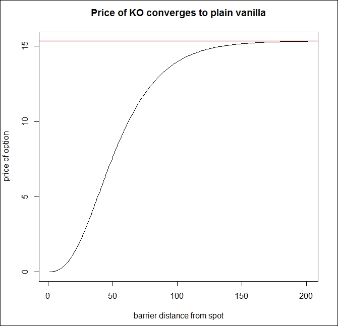
Similarly, double barrier options converge into single barrier ones if one of the barriers starts to get unimportant and converges towards plain vanillas if both the barriers are getting unimportant.

Thanks to the preceding mentioned parities, most of the time, finding pricing formulas for KO options is enough. Although this is of huge help, often, pricing a KO could be still very tricky. Replicating the KO event is based on a technique that tries to build a portfolio made of vanillas that have exactly zero worth when the knock event occurs, so at that point, they can be closed for free. There are two famous methods for this, explained by Derman-Ergener-Kani (1995) and Carr-Ellis-Gupta (1998).

The so-called Black-Scholes surface is a 3D chart where the option price can be shown as a function of time to maturity and the underlying price. Since some of the exotic pricing functions can go crazy under extreme input circumstances, it is advisable to use our financial knowledge that an option price can never go below zero.

The following is the code for the Black-Scholes surface:

install.packages('plot3D')
BS_surface <- function(S, Time, FUN, ...) {
    require(plot3D)
    n <- length(S)
    k <- length(Time)
    m <- matrix(0, n, k)
    for (i in 1:n){
        for (j in 1:k){
            l <- list(S = S[i], Time = Time[j], ...)
             m[i,j] <- max(do.call(FUN, l)@price, 0)
        }
    }
    persp3D(z = m, xlab = "underlying", ylab = "Remaining time",
        zlab = "option price", phi = 30, theta = 20, bty = "b2")
}
BS_surface(seq(1, 200,length = 200), seq(0, 2, length = 200),
    GBSOption, TypeFlag = "c", X = 90, r = 0.02, b = 0, sigma = 0.3)

The preceding code yields the following output:

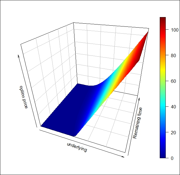
First, we prepared the Black-Scholes surface of a plain vanilla call option. However, the BS_surface code can be used for many more purposes. Just like the fact that the concept of the Black-Scholes surface can be used for any kind of single underlying dependent derivative, if we have a pricing function, it can be used as the FUN argument:

BS_surface(seq(1,200,length = 200), seq(0, 2, length = 200),
    StandardBarrierOption, TypeFlag = "cuo", H = 130, X = 90, K = 0,
    r = 0.02, b = -0.02, sigma = 0.30)

The following screenshot is the result of the preceding code:

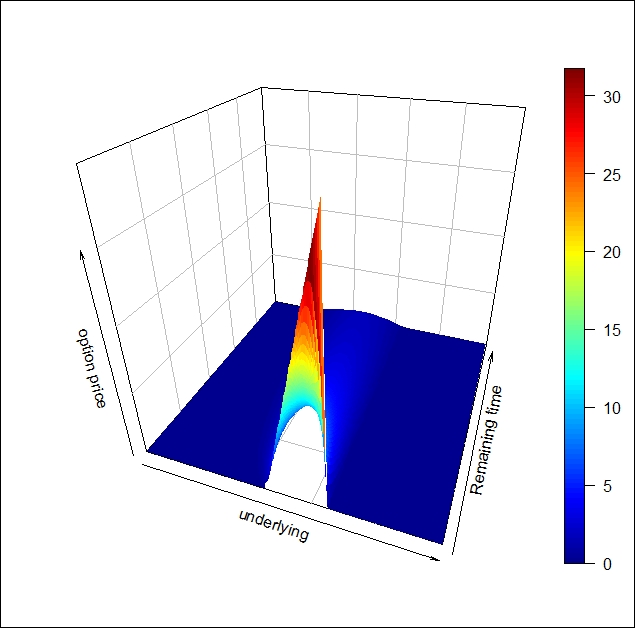
It is easy to see that compared to the plain vanilla call, the up-and-out call option has a limited value.

On [page 156], we use this same function to chart the BS Surface for a Double-no-touch option.

Binary options are exotics that have a fixed contingent payout. The name comes from the feature that they have only two possible outcomes: either pay a fixed amount or don't pay at all. They have the 0-1 relationship in the options world. Binary features could be mixed with the barrier feature; thus, they become path dependent. A One-Touch (OT) option pays only if a knock event occurred during its lifetime, while a No-Touch pays only if no knock event occurred.

There could be two barriers associated with the binaries, thus getting the Double-One-Touch and Double-No-Touch options. Based on no arbitrage arguments, the following equations must hold:

NT + OT = T-Bill

DNT + DOT = T-Bill

Convergence can be seen here too, similar to the cases we have shown for the barriers. A DNT converges to an NT if one of the barriers is far enough, and converges to a T-Bill if both the barriers are far enough. A pricing function for a DNT is the Jack-of-all-trades of the binaries, similar to the DKO option for the barrier type.

Lookback options are also path dependent. The lookback feature is very convenient. At expiry, the holder of the position can look back and choose the best price from the path of the underlying. For a floating rate lookback, the option holder can look back for the strike price. For a fixed rate lookback, the holder can exercise the option against any price on which the underlying was traded during the lifetime of the option. Taleb (1997) shows how lookbacks can be replicated by an infinite chain of KIKO options. In this sense, this is at least second generation exotic, since we need exotics as building blocks to be able to replicate a lookback.

More than one underlying is also a common exotic feature. Two examples have already been discussed in the exchange options and quanto options sections of Chapter 5, FX Derivatives. However, there are plenty more. Best-of and worst-of (also called rainbow) options are give the best or the worst performing underlying from a basket. The spread option is very similar to a vanilla option with the twist that the underlying of this option is the difference of two assets. These are just a few examples, which are enough to show that not surprisingly, in all of these cases, correlation plays an important role. Also, these features can be mixed with barrier or lookback or Asian features that result in an almost endless number of combinations. In this chapter, we will not be discussing these types any further.