
Contrary to the previous points, let us suppose that there are a finite number of risky assets available on the market. These assets are traded continuously without any transaction costs. The investor analyses historical market data and based on this, can reset her portfolio at the end of each day. How can she maximize her wealth in the long run? If returns are independent in time, then markets are efficient in the weak sense and the time series of returns have no memory. If returns are also identically distributed (i.i.d), the optimal strategy is to set portfolio weights for example, according to the Markowitz model (see Daróczi et al. 2013) and to keep portfolio weights fixed over the whole time horizon. In this setting, any rearrangements would have negative effects on the portfolio value in the long run.
Now, let us suspend the assumption of longitudinal independency, hence let us allow for hidden patterns in the asset returns, therefore markets are not efficient and it is worth analyzing historical price movements. The only assumption we keep is that asset returns are generated by a stationary and ergodic process. It can be shown that the best choice is the so called logoptimal portfolio, see Algoet-Cover (1988). More precisely, there are no other investment strategies which have asymptotically higher expected return than the logoptimal portfolio. The problem is that in order to determine logoptimal portfolios one should know the generating process.
But, what can we do in a more realistic setting when we know nothing about the nature of the underlying stochastic process? A strategy is called universally consistent if it ensures that asymptotically the average growth rate approximates that of the logoptimal strategy for any (!) generating process being stationary and ergodic. It is surprising, but universally consistent strategies exist, see Algoet-Cover (1988). Thus, the basic idea is to search for patterns in the past that are similar to the most recently observed pattern, and building on this, to forecast the future returns and to optimize the portfolio relative to this forecast. The concept of similarity can be defined in different ways, therefore we can use different approaches, for example partitioning estimator, core function based estimator and nearest neighbor estimator. For illustration purposes, in the next point we present a simple universally consistent strategy which is based on the core function approach according to Györfi et al. (2006).
Let us suppose that there are d different stocks traded on the market. Vector b containing portfolio weights can be rearranged every day. We suppose that portfolio weights are nonnegative (short selling is not allowed) and the sum of the weights is always 1 (the portfolio must be self-financing). Vector x contains price relatives ![]() where P stands for the closing price on the ith day. The investor's initial wealth is S0, hence her wealth at the end of the nth period is as follows:
where P stands for the closing price on the ith day. The investor's initial wealth is S0, hence her wealth at the end of the nth period is as follows:
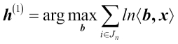
where ![]() is the scalar product of the two vectors, n is the number of the days we followed the investment strategy, Wn is the average log return over the n days and B represents all the b vectors applied. Therefore, the task is to determine a reallocation rule in a way that Wn be maximal in the long run. Here we present a simple universally consistent strategy which disposes this attractive property. Let Jn denote the set of days which are similar to the most recently observed day in terms of the Euclidean distance. It is determined by the formula
is the scalar product of the two vectors, n is the number of the days we followed the investment strategy, Wn is the average log return over the n days and B represents all the b vectors applied. Therefore, the task is to determine a reallocation rule in a way that Wn be maximal in the long run. Here we present a simple universally consistent strategy which disposes this attractive property. Let Jn denote the set of days which are similar to the most recently observed day in terms of the Euclidean distance. It is determined by the formula
where rl is the maximum allowed distance (radium) selected by the lth expert. The logoptimal portfolio according to the lth expert on day n can be expressed in the following way:
In order to get a well-balanced and robust strategy we define different experts (portfolio managers) with different radium, and we allocate our wealth to different experts according to a weight vector q. Weights can be equal; or can depend on the previous performance of the experts or on other characteristics. This way we combine the opinion of several experts and our wealth on the nth day is
Let us suppose that we are an expert and we follow the above strategy between 1997 and 2006 on the market of four NYSE stocks (aph, alcoa, amerb, and coke) plus a U.S. treasury bond and we use a moving time-window of one year. Data can be collected for example from here: http://www.cs.bme.hu/~oti/portfolio/data.html. Let us first read the data in.
all_files <- list.files("data")
d <- read.table(file.path("data", all_files[[1]]),
       sep = ",", header = FALSE)
colnames(d) = c("date", substr(all_files[[1]], 1, nchar(all_files[[1]]) - 4))
for (i in 2:length(all_files)) {
  d2 <- read.table(file.path("data", all_files[[i]]), sep = ",", header = FALSE)
  colnames(d2) = c("date", substr(all_files[[i]], 1, nchar(all_files[[i]])-4))
  d <- merge(d, d2, sort = FALSE)
}
This function calculates the expected value of the portfolio in line with the portfolio weights depending on the radium (r) we set in advance.
log_opt <- function(x, d, r = NA) {
  x <- c(x, 1 - sum(x))
  n <- ncol(d) - 1
  d["distance"] <- c(1, dist(d[2:ncol(d)])[1:(nrow(d) - 1)])
  if (is.na(r)) r <- quantile(d$distance, 0.05)
  d["similarity"] <- d$distance <= r
  d["similarity"] <- c(d[2:nrow(d), "similarity"], 0)
  d <- d[d["similarity"] == 1, ]
  log_return <- log(as.matrix(d[, 2:(n + 1)]) %*% x)
  sum(log_return)
}
This function calculates the optimal portfolio weights for a particular day.
log_optimization <- function(d, r = NA) {
  today <- d[1, 1]
  m <- ncol(d)
  constr_mtx <- rbind(diag(m - 2), rep(-1, m - 2))
  b <- c(rep(0, m - 2), -1)
  opt <- constrOptim(rep(1 / (m - 1), m - 2), function(x) -1 * log_opt(x, d), NULL, constr_mtx, b)
  result <- rbind(opt$par)
  rownames(result) <- today
  result
}
Now we optimize the portfolio weight for all the days we found similar. At the same time we also calculate the actual value of our investment portfolio for each day.
simulation <- function(d) {
  a <- Position( function(x) substr(x, 1, 2) == "96", d[, 1])
  b <- Position( function(x) substr(x, 1, 2) == "97", d[, 1])
  result <- log_optimization(d[b:a,])
  result <- cbind(result, 1 - sum(result))
  result <- cbind(result, sum(result * d[b + 1, 2:6]), sum(rep(1 / 5, 5) * d[b + 1, 2:6]))
  colnames(result) = c("w1", "w2", "w3", "w4", "w5", "Total return", "Benchmark")
  for (i in 1:2490) {
    print(i)
    h <- log_optimization(d[b:a + i, ])
    h <- cbind(h, 1 - sum(h))
    h <- cbind(h, sum(h * d[b + 1 + i, 2:6]), sum(rep(1/5,5) * d[b + 1 + i, 2:6]))
    result <- rbind(result,h)
  }
  result
}
A <- simulation(d)
Finally, let us plot the investment value in time.
matplot(cbind(cumprod(A[, 6]), cumprod(A[, 7])), type = "l",
  xaxt = "n", ylab = "", col = c("black","grey"), lty = 1)
legend("topright", pch = 19, col = c("black", "grey"),
  legend = c("Logoptimal portfolio", "Benchmark"))
axis(1, at = c(0, 800, 1600, 2400), lab = c("1997-01-02", "2001-03-03", "2003-05-13", "2006-07-17"))
We got the following graph:
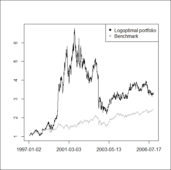
We can see on the above graph that our log-optimal strategy outperformed the passive benchmark of keeping portfolio weights equal and fixed over time. However, it is notable that not only the average return, but also the volatility of the investment value is much higher in the former case.
It is mathematically proven that there exist non-parametric investment strategies which are able to effectively reveal hidden patterns in the realized returns and to exploit them in order to achieve an "almost" optimal growth rate in the investor's wealth. For this, we do not have to know the underlying process; the only assumption is that the process is stationary and ergodic. However, we cannot be sure that this assumption holds in reality. It is also important to emphasize that these strategies are optimal only in the asymptotic sense, but we know little about the short run characteristics of the potential paths.