
As we shown earlier, increasing the number of portfolio adjustments leads to a decrease in the volatility of the hedging cost. As Δt approaches 0, the cost of hedging approximates the option price derived from the BS formula. Until now, we have disregarded the transaction costs, but here, we remove this assumption and analyze the effects of transaction costs on option hedging. As rebalancing becomes more frequent, transaction costs increase the cost of hedging, but at the same time, shorter rebalancing periods reduce the volatility of the hedging cost. Hence, it is worth examining this trade-off in more detail, and based on this, defining the optimal rebalancing strategy. An absolute (fixed for each transaction) or a relative (proportional to the transaction size) transaction cost can be added to the code by modifying the parameters when we define the function:
cost_simulation = function(S0, mu, sigma, rf, K, Time, dt, periods, cost_per_trade)
Then, the cost calculation method for the absolute transaction cost can be programmed as follows:
share_cost[1] <- S[1]*delta[1] + cost_per_trade
interest_cost[1] <- (exp(rf*dt*periods)-1) * share_cost[1]
total_cost[1] <- share_cost[1] + interest_cost[1]
for(i in 2:m){
    share_cost[i] <- ( delta[i] - delta[i-1] ) * S[i] + cost_per_trade
    interest_cost[i] <- ( total_cost[i-1] + share_cost[i] ) * (exp(rf*dt*periods)-1)
    total_cost[i] <- total_cost[i-1] + interest_cost[i] + share_cost[i]
             }
In the case of relative costs, the program code is as follows:
share_cost[1] <- S[1]*delta[1]*(1+trading_cost)
interest_cost[1] <- (exp(rf*dt*periods)-1) * share_cost[1]
total_cost[1] <- share_cost[1] + interest_cost[1]
for(i in 2:m){
    share_cost[i] <- (( delta[i] - delta[i-1] ) * S[i]) + abs(( delta[i] - delta[i-1] ) * S[i]) * trading_cost
    interest_cost[i] <- ( total_cost[i-1] + share_cost[i] ) * (exp(rf*dt*periods)-1)
    total_cost[i] <- total_cost[i-1] + interest_cost[i] + share_cost[i]
}
When referring to the cost_simulation function, the absolute or relative cost has to be given. Let's check the effect of an absolute cost of 0.02 per transaction (we suppose that the unit of the cost and the extent of the trade are the same). In order to shorten the time consumption, we used only 100 simulated paths here.
We have to change the parameters of the cost_simulation function in the cycle:
for (i in 1:100)
  A[i] = cost_simulation(100, .20, .30,.05, 100, 0.5, 1/1000,j,.02)
Then, we get the table shown as follows:
                 E     lower   upper          v      ratio
1/2 days 12.083775 11.966137 12.20141 0.6001933 0.06229386
1 day    10.817594 10.643468 10.99172 0.8883994 0.09220668
2 days   10.244342  9.999395 10.48929 1.2497261 0.12970866
1 week    9.993442  9.612777 10.37411 1.9421682 0.20157700
2 weeks  10.305498  9.737017 10.87398 2.9004106 0.30103266
4 weeks  10.321880  9.603827 11.03993 3.6635388 0.38023748
Calculating with a fixed transaction cost of 0.02, the expected value of the hedging cost increases considerably. The shorter rebalancing periods are most affected as more trading enhances the costs. The standard deviation is also higher, mainly in cases of periods shorter than one week.
We can see the effect of the relative transaction cost of 1 percent by applying the following change in the code:
for (i in 1:100)
  A[i] = cost_simulation(100, .20, .30,.05, 100, 0.5, 1/1000,j, 0.01)
The expected hedging cost has increased further in the case of the shortest (daily or even more frequent) rebalancing periods, but we also found a more significant rise of the volatility (as shown in the following output table):
                E    lower    upper         v     ratio
1/2 days 13.56272  13.26897  13.85646 1.498715 0.1555512
1 day    12.53723  12.28596  12.78850 1.282005 0.1330589
2 days   11.89854  11.59787  12.19921 1.534010 0.1592144
1 week   11.37828  10.96775  11.78880 2.094506 0.2173881
2 weeks  11.55362  10.95111  12.15612 3.073993 0.3190487
4 weeks  11.43771  10.69504  12.18038 3.789128 0.3932724
The presence of transaction costs offsets the volatility reduction effect of the more frequent rebalancing, so the optimal rebalancing period is to be determined by weighting these effects relative to each other.
In order to find the optimal length of the rebalancing period, we have to define the optimization criterion and the measure that is to be maximized or minimized. The usual aim of hedging is the reduction of the risk, measured by the variance of the cost of the hedge. According to this, the optimal hedge minimizes the volatility of the cost of hedging. Another aim of the optimization can be the minimization of the expected value of the cost. As we have seen, in the absence of transaction costs, these goals can be achieved simultaneously by rebalancing the hedging portfolio more and more frequently. On the other hand, transaction costs boost not only the expected value of the cost but also the volatility, which can rise drastically when the readjustment is too frequent.
It is a widespread method in finance when trade-off between the expected value and volatility has to be considered in order to define a utility function and an optimum as the maximum utility. For example, in the portfolio theory, an individual utility function is assumed, which is positively affected by the expected value of the return and negatively affected by its variance. We can use the same technique by defining a utility function that contains the expected value of the cost of hedging and its variance. However, in our case, both factors have a negative impact on the utility of the trader; therefore, both parameters must have a positive sign, and the function is to be minimized. Accordingly, the objective function will be a utility function defined as follows:
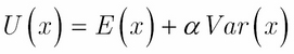
Equation 3
Here, x is the cost of the hedge as a random variable, E denotes its expected value, Var stands for its variance, and α is the risk aversion parameter. A higher α indicates a more risk averse investor/trader.
An alternative solution to the mean-variance optimization can be setting the expected (cost) value minimization as the main goal with the boundary condition that keeps a chosen risk measure under a predefined value. Here, we chose Value-at-Risk as the control variable, which is a type of downside risk measure, defined as the maximal loss or worst outcome at a predefined probability and over a selected time horizon.
The following code calculates the cost distribution based on 1,000 simulations for different rebalancing periods from 1-80 Δt. The unit of Δt is a quarter of a day, so Δt of 1 means four readjustments a day; the longest Δt of 80 refers to a 20-day long period. The function collects the expected value, the standard deviation, and the 95 percentile of the distribution, and gives the result of the four different optimization scenarios in text format and also plots the results:
n_sim <- 1000
threshold <- 12
cost_Sim <- function(cost = 0.01, n = n_sim, per = 1){a <- replicate(n, cost_simulation(100, .20, .30,.05, 100, 0.5, 1/1000,per,cost));
l <- list(mean(a), sd(a), quantile(a,0.95))}
A <- sapply(seq(1,80) ,function(per) {print(per); set.seed(2019759); cost_Sim(per = per)})
e <- unlist(A[1,])
s <- unlist(A[2,])
q <- unlist(A[3,])
u <- e + s^2
A <- cbind(t(A), u)
z1 <- which.min(e)
z2 <- which.min(s)
z3 <- which.min(u)
    (paste("E min =", z1, "cost of hedge = ",e[z1]," sd = ", s[z1]))
    (paste("s min =", z2, "cost of hedge = ",e[z2]," sd = ", s[z2]))
    (paste("U min =", z3, "u = ",u[z3],"cost of hedge = ",e[z3]," sd = ", s[z3]))
matplot(A, type = "l", lty = 1:4, xlab = "Δt", col = 1)
lab_for_leg = c("E", "Sd", "95% quantile","E + variance")
legend(legend = lab_for_leg, "bottomright", cex = 0.6, lty = 1:4)
abline( v = c(z1,z2,z3), lty = 6, col = "grey")
abline( h = threshold, lty = 1, col = "grey")
text(c(z1,z1,z2,z2,z3,z3,z3),c(e[z1],s[z1],s[z2],e[z2],e[z3],s[z3],u[z3]),round(c(e[z1],s[z1],s[z2],e[z2],e[z3],s[z3],u[z3]),3), pos = 3, cex = 0.7)
e2 <- e
e2[q > threshold] <- max(e)
z4 <- which.min(e2)
z5 <- which.min(q)
if( q[z5] < threshold ){
print(paste(" min VaR = ", q[z4], "at", z4 ,"E(cost | VaR < threshold = " ,e[z4], " s = ", s[z4]))
 } else {
    print(paste("optimization failed, min VaR = ", q[z5], "at", z5 , "where cost = ", e[z5], " s = ", s[z5]))
             }
The last optimization searches for the minimal cost that can be achieved with the condition that Value-at-Risk at the q significance level (the q percentile) does not exceed the predetermined threshold. As it is not necessary that this minimum exists, if the optimization fails, the minimum of q-VaR is given as the result.
The task is to find the optimal length of the rebalancing period in the case of transaction costs and for a vanilla call option with the already investigated parameters. Let's suppose that the transaction cost is 0.01 per trade.
The output of the earlier function is a matrix A that contains the parameters of the distribution that belong to different rebalancing periods, and the optimum according to different criteria.
The first and last rows of the matrix A are shown next:
     [,1]     [,2]      [,3]     [,4]
 [1,] 14.568   0.3022379 15.05147 14.65935
 [2,] 12.10577 0.4471673 12.79622 12.30573
...
 [79,] 10.00434 2.678289  14.51381 17.17757
 [80,] 10.03162 2.674291  14.41796 17.18345
The number in the square brackets stands for the rebalancing period expressed in Δt. The next columns contain the expected value, the standard deviation, the 95 percent quantile, and the sum of the expected value and standard deviation. The results of the four optimization processes are summarized in the next output:
"E min = 50 cost of hedge =  9.79184040508574  sd =  2.21227796458088"
"s min = 1 cost of hedge =  14.5680033393436  sd =  0.302237879069942"
"U min = 8 u =  11.0296321604941 cost of hedge =  10.2898541853535  sd =  0.860103467694771"
" min VaR =  11.8082026178249 at 14 E(cost | VaR < threshold =  10.0172915117802  s =  1.12757856083913"
The following figure depicts the results in the function of the rebalancing periods (in Δt). The dashed line shows the standard deviation and the solid line is the expected cost, while the dot dash and dotted lines stand for the value of the utility function (Equation 3) with an alpha parameter of 1 and 95 percentile respectively.
Although the optimization depends on the parameters, the chart illustrates the trade-off between the expected cost and the volatility in the presence of transaction costs:
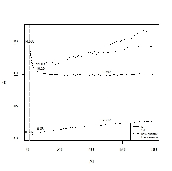
The minimum of the expected cost (9.79) is not far away from the BS price of 9.63. The optimal rebalancing period is then 50 Δt, that is, 12.5 days long. At the lowest expected cost, the standard deviation is 2.21.
The volatility minimization results in the most frequent rebalancing, which means rebalancing 4 times a day; then, the minimum of the standard deviation is 0.30, but the frequent trading increases the costs drastically. The expected cost is 14.57, which is about 50 percent higher than in the previous case.
The optimization model based on the utility function defined in Equation 3 considers both aspects of the hedge, and the earlier output shows 8 Δt long rebalancing periods as optimal, that is, exactly 2 days. We can achieve an expected value of 10.29, which only somewhat exceeds the minimum, and the standard deviation is 0.86.
The last row of the preceding output presents the results of the optimization using Value-at-Risk limits. We applied a 95% VaR and searched for the minimal expected cost at which, in 95% of the cases, the cost remains under a threshold of 12. According to this, the optimal length of the readjustment is 14 Δt, that is, 3.5 days. The expected value of the cost is slightly lower (10.02) than in the previous case, where the result is offset by a slightly higher standard deviation (1.13).
In this section, the same optimization problem is solved as in the previous section, with the exception that now the transaction cost is 1 percent of the deal. All other parameters are the same.
The output contains the matrix A with the same data:
      [,1]     [,2]     [,3]     [,4]
 [1,] 16.80509 2.746488 21.37177 24.34829
 [2,] 14.87962 1.974883 18.20097 18.77978
...
 [79,] 11.2743  2.770777 15.89386 18.9515
 [80,] 11.31251 2.758069 16.0346  18.91945
Given that costs depend on the transaction size, we got a U-shape not only in the expected value, but also in the standard deviation. This indicates that too frequent trading is suboptimal also in regards to volatility minimization.
The other main difference compared to the previous optimization is that the threshold of VaR cannot be held (as shown in the following code):
"E min = 56 cost of hedge =  11.1495374978655  sd =  2.40795704676431"
"s min = 9 cost of hedge =  12.4747301348104  sd =  1.28919873150291"
"U min = 14 u =  13.9033123535802 cost of hedge =  12.0090095949856  sd =  1.37633671701175"
"optimization failed, min VaR =  14.2623891995575 at 21 where cost =  11.7028044352096  s =  1.518297863428"
The following screenshot gives the output of the preceding command:
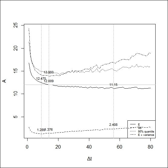
The lowest expected cost is 11.15 with a standard deviation of 2.41 at 56 Δt, indicating an optimal rebalancing period of 14 days.
The lowest volatility is 1.23 at Δt of 9, and the expected value is 12.47. The mean-variance optimization results in a rebalancing period of 14 Δt (3.5 days), the standard deviation is 1.38, and the expected value is 12.01.
As mentioned, the fourth optimization fails; the minimum of the 95% VaR is 14.26, which can be achieved at 21 Δt (5.25 days); the expected cost is 11.7, and the standard deviation is 1.52.
The optimization shows that in the presence of the transaction cost, the simple aim of volatility reduction causes a huge rise in the costs; therefore, an optimal hedging strategy has to take into consideration this effect as well.