
After remaining a long time in academic circles due to their advanced mathematical background, neural networks (NN) rapidly grew in popularity as more practically usable formats are available – like the built-in function of R. NNs are artificial intelligence adaptive software that can detect complex patterns in data: it is just like an old trader who has a good market intuition but cannot always explain to you why he is convinced you should go short on the Dow Jones Industrial Average index (DIJA).
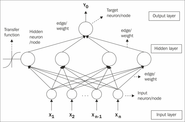
The network architecture consists of a number of nodes connected by links. Networks usually have 3 or 4 layers: input, hidden and output layers, and in each layer several neurons can be found. The number of first layer's nodes corresponds to the number of the model's explanatory variables, while the last layer's equals to the number of the response variables (usually 2 neurons in case of binary target variable or 1 neuron in case of continuous target variable). The model's complexity and forecast ability is determined by the number of nodes in the hidden layer(s). Normally, each node of one layer has connections to all the other nodes of the next layer, and these edges (see the figure) represent weights. Every neuron receives inputs from the previous layer and, by the use of a non-linear function, it transforms to the next layer's input.
A feed-forward NN with one hidden layer can be useful almost in case of any kind of complex problems (Chauvin-Rumelhart, 1995), that is why it often used by researchers. (Sermpinis et al., 2012; Dai et al, 2012) Atsalakis-Valavanis (2009) pointed out, that the multi-layer precepton (MLP) model that belongs to the family of feed-forward neural networks (FFNN) can be the most effective to forecast financial time series. The next graph depicts the structure of a 3 layer MLP neural network, according to (Dai et al, 2012).
The connection weights (the values of the edges) are assigned initial values first. The error between the predicted and actual output values is back-propagated via the network for updating the weights. The supervised learning procedure then attempts to minimize the error (usually MSE, RMSE or MAPE) between the desired and forecasted outputs. Since the network with certain number of neurons in the hidden layer can learn any relationship on the learning data (even the outliers and noise), by halting the learning algorithm early the prevention of the over-learning is possible. The learning process of the network stops when the test segment has reached its minimum. Then, with the given parameter the network has to be run on the validation segment, see (Wang et al., 2012).
There are many practical problems to solve when you create and perform your own neural network, for example, the selection of appropriate network topology, the selection and the transformation of input variables, the reduction of output variance and most importantly the mitigation of over fitting which refers to the situation when the error on the training set is very small, but when we fit the network on new data the error is large. It means that the network has just memorized the training examples but was not successful in understanding the general structure of the relationships. In order to avoid overfitting, we need to split the data into three subsets: train, validation, test. The training set usually accounting for the 60-70% of the total data is used for learning and fitting the network parameters. The validation data set (10-20%) is used for minimizing the overfitting effect and tuning the parameters, for example to choose the number of hidden nodes in a NN. The test data (10-20%) set is used only for testing the final solution in order to confirm the predictive power of the network.
Let us see how it works in practice. This example applies trading strategies based on the forecasting of the closing prices of Bitcoin. The period between 3 August 2013 and 8 May 2014 were selected for analysis. There were totally 270 data points in the dataset and the first 240 data points was used as the training sample while the remaining 30 points was used as the testing sample (the forecasting models were tested on the last one months of this time series of 9 months).
First we load the dataset from Bitcoin.csv which can be found on the website of the book.
data <- read.csv("Bitcoin.csv", header = TRUE, sep = ",")
data2 <- data[order(as.Date(data$Date, format = "%Y-%m-%d")), ]
price <- data2$Close
HLC <- matrix(c(data2$High, data2$Low, data2$Close), nrow = length(data2$High))
In the second step we calculate the log returns and install the TTR library in order to generate technical indicators.
bitcoin.lr <- diff(log(price))
install.packages("TTR")
library(TTR)
The six technical indicators selected for modeling have been widely and successfully used by researchers and professional traders as well.
rsi    <- RSI(price)
MACD   <- MACD(price)
macd   <- MACD[, 1]
will   <- williamsAD(HLC)
cci    <- CCI(HLC)
STOCH  <- stoch(HLC)
stochK <- STOCH[, 1]
stochD <- STOCH[, 1]
We create the Input and Target matrix for training and validation dataset. The training and validation dataset include the closing prices and technical indicators between August 3, 2013 (700) and April 8, 2014 (940).
Input <- matrix(c(rsi[700:939], cci[700:939], macd[700:939],will[700:939], stochK[700:939], stochD[700:939]), nrow = 240)
Target <- matrix(c(bitcoin.lr[701:940]), nrow = 240)
trainingdata <- cbind(Input, Target)
colnames(trainingdata) <- c("RSI", "CCI", "MACD", "WILL", "STOCHK", "STOCHD", "Return")
Now, we install and load the caret package order to split our learning dataset.
install.packages("caret")
library(caret)
We split the learning dataset in 90-10% (train-validation) ratio.
trainIndex <- createDataPartition(bitcoin.lr[701:940], p = .9, list = FALSE)
bitcoin.train <- trainingdata[trainIndex, ]
bitcoin.test <- trainingdata[-trainIndex, ]
We install and load the nnet package.
install.packages("nnet")
library(nnet)
The appropriate parameters (number of neurons in hidden layer, learning rate) are selected by means of the grid search process. The network's input layer comprise six neurons (in accordance with the number of explanatory variables), whereas networks of 5, 12, …, 15 neurons were tested in the hidden layer. The network has one output: the daily yield of the bitcoin. The models were tested at low learning rates (0.01, 0.02, 0.03) in the learning process. The convergence criterion used was a rule that the learning process would be halted if the 1000th iteration has been reached. The network topology with the lowest RMSE in the test set was chosen as optimal.
best.network <- matrix(c(5, 0.5))
best.rmse <- 1
for (i in 5:15)
  for (j in 1:3) {
    bitcoin.fit <- nnet(Return ~ RSI + CCI + MACD + WILL + STOCHK + STOCHD, data = bitcoin.train, maxit = 1000, size = i, decay = 0.01 * j, linout = 1)
    bitcoin.predict <- predict(bitcoin.fit, newdata = bitcoin.test)
    bitcoin.rmse <- sqrt(mean ((bitcoin.predict – bitcoin.lr[917:940])^2))
    if (bitcoin.rmse<best.rmse) {
      best.network[1, 1] <- i
      best.network[2, 1] <- j
      best.rmse <- bitcoin.rmse
    }
  }
In this step, we create the Input and Target matrix for the test dataset. The test dataset include the closing prices and technical indicators between April 8, 2013 (940) and May 8, 2014 (969).
InputTest <- matrix(c(rsi[940:969], cci[940:969], macd[940:969], will[940:969], stochK[940:969], stochD[940:969]), nrow = 30)
TargetTest <- matrix(c(bitcoin.lr[941:970]), nrow = 30) Testdata <- cbind(InputTest,TargetTest)
colnames(Testdata) <- c("RSI", "CCI", "MACD", "WILL", "STOCHK", "STOCHD", "Return")
Finally, we fit the best neural network model on test data.
bitcoin.fit <- nnet(Return ~ RSI + CCI + MACD + WILL + STOCHK + STOCHD, data = trainingdata, maxit = 1000, size = best.network[1, 1], decay = 0.1 * best.network[2, 1], linout = 1)
bitcoin.predict1 <- predict(bitcoin.fit, newdata = Testdata)
We repeat and average the model 20 times in order to eliminate the outlier networks.
for (i in 1:20) {
  bitcoin.fit <- nnet(Return ~ RSI + CCI + MACD + WILL + STOCHK + STOCHD, data = trainingdata, maxit = 1000, size = best.network[1, 1], decay = 0.1 * best.network[2, 1], linout = 1)
  bitcoin.predict <- predict(bitcoin.fit, newdata = Testdata)
  bitcoin.predict1 <- (bitcoin.predict1 + bitcoin.predict) / 2
}
We calculate the result of the buy-and-hold benchmark strategy and neural network on the test dataset.
money <- money2 <- matrix(0,31)
money[1,1] <- money2[1,1] <- 100
for (i in 2:31) {
  direction1 <- ifelse(bitcoin.predict1[i - 1] < 0, -1, 1)
  direction2 <- ifelse(TargetTest[i - 1] < 0, -1, 1)
  money[i, 1] <- ifelse((direction1 - direction2) == 0, money[i-1,1]*(1+abs(TargetTest[i - 1])),
      money[i-1,1]*(1-abs(TargetTest[i - 1])))
  money2[i, 1] <- 100 * (price[940 + I - 1] / price[940])
}
We plot the investment value according to the benchmark and the neural network strategy on the test dataset (1 month).
x <- 1:31
matplot(cbind(money, money2), type = "l", xaxt = "n",
  ylab = "", col = c("black", "grey"), lty = 1)
legend("topleft", legend = c("Neural network", "Benchmark"),
  pch = 19, col = c("black", "grey"))
axis(1, at = c(1, 10, 20, 30),
  lab = c("2014-04-08", "2014-04-17", "2014-04-27", "2014-05-07"))
box()
mtext(side = 1, "Test dataset", line = 2)
mtext(side = 2, "Investment value", line = 2)
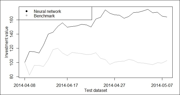
We note that in this illustrative example NN strategy has outperformed the "buy-and-hold" strategy in terms of the realized return. With neural network we achieved a return of 20% in a month, while with the passive buy and hold strategy it was only 3%. However, we didn't take into account the transaction costs, the bid-ask spreads and the price impacts and these factors may reduce the neural network's profit significantly.