The Vasicek model (Vasicek, 1977) is a continuous, affine, one-factor stochastic interest rate model. In this model, the instantaneous interest rate dynamics are given by the following stochastic differential equation:

Here, α, β, and σ are positive constants, r_t is the interest rate, t is time, and W_t denotes the standard Wiener process. In mathematics, this process is called the Ornstein-Uhlenbeck process.

As you may observe, the interest rate in the Vasicek model follows a mean-reverting process with a long-term average β; when r_t < β, the drift term becomes positive, so the interest rate is expected to increase and vice versa. The speed of adjustment to the long-run mean is measured by α. The volatility term is constant in this model.

Interest rate models are implemented in R, but to understand more deeply what is behind the formulas, let's write a function that directly implements the stochastic differential equation of the Vasicek model:

vasicek <- function(alpha, beta, sigma, n = 1000, r0 = 0.05){
  v <- rep(0, n)
  v[1] <- r0
  for (i in 2:n){
    v[i] <- v[i - 1] + alpha * (beta - v[i - 1]) + sigma * rnorm(1)
         }
     return(v)
}

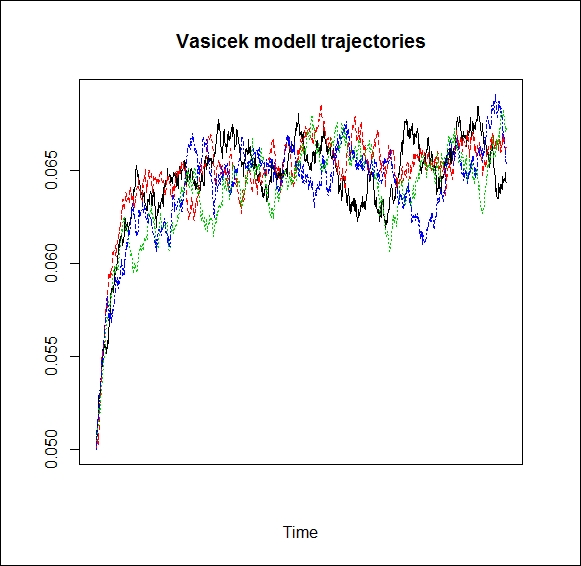
That's it. Now, let's plot some trajectories to see how it looks:

set.seed(123)
r <- replicate(4, vasicek(0.02, 0.065, 0.0003))

matplot(r, type = "l", ylab = "", xlab = "Time", xaxt = "no",  main = "Vasicek modell trajectories")
lines(c(-1,1001), c(0.065, 0.065), col = "grey", lwd = 2, lty = 1)

The following screenshot gives the output of the preceding command:

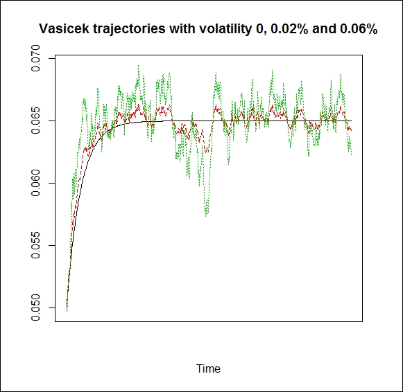
To understand the role of parameters, we plot the same trajectory (that is, the trajectory generated by the same random numbers) with different values of sigma and alpha:

r <- sapply(c(0, 0.0002, 0.0006), 
function(sigma){set.seed(102323); vasicek(0.02, 0.065, sigma)})

matplot(r, type = "l", ylab = "", xlab = "Time" ,xaxt = "no",  main = "Vasicek trajectories with volatility 0, 0.02% and 0.06%")
lines(c(-1,1001), c(0.065, 0.065), col = "grey", lwd = 2, lty = 3)

The following is the output of the preceding code:

r <- sapply(c(0.002, 0.02, 0.2),
function(alpha){set.seed(2014); vasicek(alpha, 0.065, 0.0002)})

Trajectories have the same shape but different volatility:

matplot(r, type = "l", ylab = "", xaxt = "no",  main = "Vasicek trajectories with alpha = 0.2%, 2% and 20%")
lines(c(-1,1001), c(0.065, 0.065), col = "grey", lwd = 2, lty = 3)

The following is the output of the preceding command:

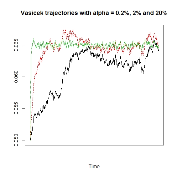
We can see that the higher the value of α, the earlier the trajectory reaches the long-term average.

It can be shown (see, for example, the original paper of Vasicek already cited) that the short rate in the Vasicek model is normally distributed with the following conditional expected value and variance:

It is worth observing that the expected value converges to β when T or α goes to infinity. Furthermore, the variance converges to 0 when α goes to infinity. These observations are in line with the parameters' interpretations.

To demonstrate how the coefficients of the equation determine the parameters of the distribution, let's plot the conditional probability density function for different values of α, β, and σ, and see how it changes over time:

vasicek_pdf = function(x, alpha, beta, sigma, delta_T, r0 = 0.05){
  e <- r0*exp(-alpha*delta_T)+beta*(1-exp(-alpha*delta_T))
  s <- sigma^2/(2*alpha)*(1-exp(-2*alpha*delta_T))
  dnorm(x, mean = e, sd = s)
}

x <- seq(-0.1, 0.2, length = 1000)
par(xpd = T ,mar = c(2,2,2,2), mfrow = c(2,2))
y <- sapply(c(10, 5, 3, 2), function(delta_T)
       vasicek_pdf(x, .2, 0.1, 0.15, delta_T))
par(xpd = T ,mar = c(2,2,2,2), mfrow = c(2,2))  
matplot(x, y, type = "l",ylab ="",xlab = "")
legend("topleft", c("T-t = 2", "T-t = 3", "T-t = 5", "T-t = 10"), lty = 1:4, col=1:4, cex = 0.7)

y <- sapply(c(0.1, 0.12, 0.14, 0.16), function(beta)
       vasicek_pdf(x, .2, beta, 0.15, 5))
matplot(x, y, type = "l", ylab ="",xlab = "")
legend("topleft", c("beta = 0.1", "beta = 0.12", "beta = 0.14", "beta = 0.16"), lty = 1:4, col=1:4,cex = 0.7)

y <- sapply(c(.1, .2, .3, .4), function(alpha)
       vasicek_pdf(x, alpha, 0.1, 0.15, 5))

matplot(x, y, type = "l", ylab ="",xlab = "")
legend("topleft", c("alpha = 0.1", "alpha = 0.2", "alpha = 0.3", "alpha = 0.4"), lty = 1:4, col=1:4, cex = 0.7)

y <- sapply(c(.1, .12, .14, .15), function(sigma)
       vasicek_pdf(x, .1, 0.1, sigma, 5))
matplot(x, y, type = "l", ylab ="",xlab = "")
legend("topleft", c("sigma = 0.1", "sigma = 0.12", "sigma = 0.14", "sigma = 0.15"), lty = 1:4, col=1:4, cex = 0.7)

The following screenshot is the result of the of preceding code:

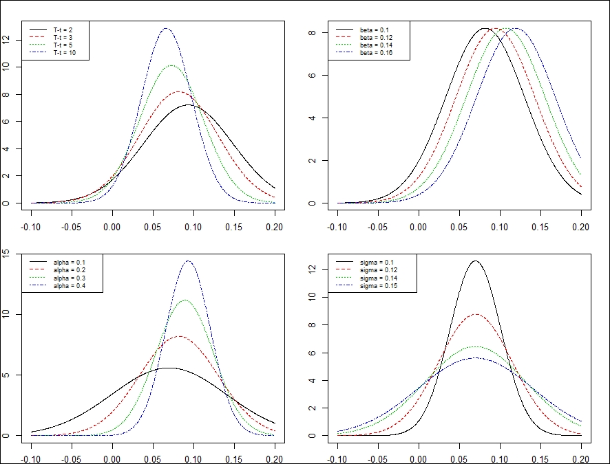
We can see that the variance of the distribution increases over time. β affects only the mean of the probability distribution. It is clear that with a higher value of α, the process reaches its long-term mean sooner and has less variance, and with greater volatility, we get a flatter density function, that is, greater variance.

Pricing a zero-coupon bond when the interest rate follows a Vasicek model results in the following formula (for a derivation of this formula, see, for example, Cairns [2004]):

Here, and .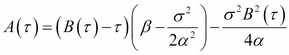

In the preceding formula, P denotes the price of the zero-coupon bond, t is the time when we price the bond, and T is the maturity (hence, T-t is the time to maturity). If we have the zero-coupon bond prices, we can determine the spot yield curve with the following simple relationship: